


Figure 4.
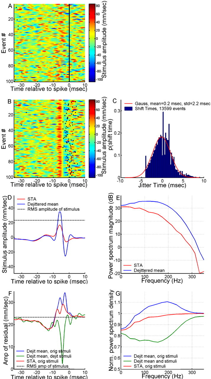
Characteristics of a dejittered mean stimulus. A, Random representative subset of 100 sample segments of stimulus-response data aligned to time of spike occurrence. The vertical black line at t = 0 is the raster plot of spikes superimposed on the color-coded traces of air-current velocity versus time. B, The same random subset of 100 segments of stimulus-response data from A but now dejittered so that their alignment is based on minimal variance of the stimuli. C, Shift times for all 13,600 samples (blue histogram) compared with a Gaussian having an STD of 2.2 ms (red line). D, STA (red trace) and dejittered mean (blue trace). The RMS amplitude of the stimulus is indicated with the dashed black line. E, Power spectra of the STA (red trace) and dejittered mean stimulus (blue trace). F, Red trace, Mean-square residual between the STA and the original (orig) stimulus segments. Blue trace, Mean-square residual between the dejittered (Dejit) mean and the original stimulus segments. Green trace, Mean-square residual between the dejittered mean and the dejittered stimulus segments. The RMS amplitude (amp) of the stimulus is indicated with the dashed black line. G, Power spectra of the residuals, normalized by power spectra of stimulus segments. Colors and abbreviations are the same as in F.