



Abstract
Changes in brain structure occur in remote regions following focal damage such as stroke. Such changes could disrupt processing of information across widely distributed brain networks. We used diffusion MRI tractography to assess connectivity between brain regions in 9 chronic stroke patients and 18 age-matched controls. We applied complex network analysis to calculate ‘communicability’, a measure of the ease with which information can travel across a network. Clustering individuals based on communicability separated patient and control groups, not only in the lesioned hemisphere but also in the contralesional hemisphere, despite the absence of gross structural pathology in the latter. In our highly selected patient group, lesions were localised to the left basal ganglia/internal capsule. We found reduced communicability in patients in regions surrounding the lesions in the affected hemisphere. In addition, communicability was reduced in homologous locations in the contralesional hemisphere for a subset of these regions. We interpret this as evidence for secondary degeneration of fibre pathways which occurs in remote regions interconnected, directly or indirectly, with the area of primary damage. We also identified regions with increased communicability in patients that could represent adaptive, plastic changes post-stroke. Network analysis provides new and powerful tools for understanding subtle changes in interactions across widely distributed brain networks following stroke.
Keywords: Brain connectivity, Diffusion weighted MRI, Tractography, Network science, Unsupervised classification
Introduction
Following a focal stroke, there are multiple ways in which the structure and function of the rest of the brain may change. The region immediately surrounding a stroke undergoes potentially reversible structural change and anterograde or retrograde degeneration of axons intersecting or connecting with a lesion site may occur. In addition to these degenerative structural changes, animal studies suggest that the brain has the capacity for potentially adaptive structural change in response to injury, including dendritic branching and synaptogenesis ( Biernaskie & Corbett, 2001 and Jones et al., 1996) and even growth of new long-range connections (Dancause et al., 2005).
Diffusion tensor imaging (DTI) (Basser et al., 1994) and tractography (Jones et al., 1999 and Mori et al., 1999) provide methods for interrogating white matter structure in vivo. Reductions in fractional anisotropy (FA), a DTI-derived measure of white matter microstructure ( Beaulieu, 2002 and Beaulieu, 2009), have been found above and below a stroke location, consistent with patterns of Wallerian and retrograde degeneration ( Pierpaoli et al., 2001 and Werring et al., 2000). DTI-based measures have been used not only to detect degeneration but also to pinpoint potentially beneficial white matter change. A recent study found that, while poorly recovered patients had reduced FA in both corticospinal tracts relative to healthy controls, well-recovered stroke patients had elevated FA relative to controls in the same regions (Schaechter et al., 2009). This observation is striking as it shows not only that white matter microstructure can be apparently improved following stroke, but also that such changes occur not just in the stroke hemisphere but also in the contralesional hemisphere. This result complements previous demonstrations of functional plasticity in the contralesional hemisphere in stroke patients ( Johansen-Berg et al., 2002 and Lotze et al., 2006) and of adaptive white matter plasticity in healthy subjects ( Keller & Just, 2009 and Scholz et al., 2009).
However, one difficulty with voxel-based assessments of structural change following stroke is the underlying assumption that regions of change will be highly co-localised across individuals. Given the heterogeneity in even carefully selected stroke populations, this approach may miss potentially interesting findings if they occur with a less consistent topography. An alternative approach to assessing structural connectivity is provided by complex network analysis. This refers to a class of mathematical tools that have been used to understand networks present in contexts as diverse as the internet, disease spread, scientific citations or protein interactions (Barabasi, 2009). These approaches have proved exceptionally powerful in characterising structural and functional brain networks (Bullmore and Sporns, 2009). Briefly, the brain is divided up according to some parcellation scheme (e.g., into cortical areas) to form the nodes of the network, then some measure of connectivity is derived between nodes (e.g., correlation in functional responses (Salvador et al., 2005), co-variation in cortical thickness (He et al., 2007) or probability of anatomical connectivity (Gong et al., 2009 and Iturria-Medina et al., 2008) to characterise network ‘edges’. Once a network has been defined in this way, various measures can be derived to describe the organisation of the network. Such measures can be relatively global, capturing network organisation by a summary value describing the connectivity of a whole brain or hemisphere, or can be related back to thenetwork in order to determine which brain regions are driving observed differences in network measures.
Complex network analysis approaches have recently been shown to be sensitive to subtle pathology in a number of neurological and neuropsychiatric disorders including Alzheimer’s Disease (He et al., 2008) and Schizophrenia (Bassett et al., 2008). In general, theaim has been to identify a network measure that allows separation of patients from healthy controls with a high degree of sensitivity and specificity. In stroke, there is less need for an imaging measure to assist with diagnosis, as conventional imaging does well in this regard. Rather, we wished to assess whether complex network analysis could be used to test the hypothesis that regions remote from the lesion site (including those in the contralesional hemisphere) undergo structural change, both degenerative and potentially adaptive, following unilateral stroke.
Here, we provide the first application of complex network analysis to the study of structural white matter changes following stroke. We used probabilistic diffusion weighted imaging tractography (Behrens et al., 2003 and Behrens et al., 2007) to study a group of chronic stroke patients following left hemisphere subcortical stroke. We derived connectivity estimates between cortical and subcortical brain regions of the left (lesioned) and right (contralesional) hemisphere and use these to derive weighted measures of ‘communicability’, a novel network measure that measures the ease with which information can flow between network nodes, using both direct and indirect paths (Crofts and Higham, 2009). By comparing connectivity and communicability between patients and controls we can test the hypothesis that changes in global or local network structure occur following stroke.
Materials and Methods
Subjects
9 chronic stroke patients (mean age 64, range: 41-83, 1 female) and 18 controls (mean age 58 years, range: 30-81 years, 7 females) participated in the study (Table 1). Patients were at least 6 months post first ischaemic or haemorrhagic left hemisphere subcortical stroke without concurrence of any other neurological condition. Healthy controls were recruited via advertisements and word of mouth. All subjects gave written informed consent to participate in accordance with the Declaration of Helsinki and local ethical approval (05/Q1607/63).
Table 1.
Patient details.
| age | sex | FM1 | stroke volume (mm3) | time post stroke (months) | |
|---|---|---|---|---|---|
| 1 | 61 | f | 24 | 7 | 7 |
| 2 | 59 | m | 42 | 9.1 | 22 |
| 3 | 67 | m | 61 | 3.5 | 36 |
| 4 | 68 | m | 59 | 32.4 | 43 |
| 5 | 69 | m | 51 | 72.9 | 21 |
| 6 | 54 | m | 50 | 1.3 | 23 |
| 7 | 83 | m | 45 | 9 | 18 |
| 8 | 41 | m | 64 | 40.73 | 8 |
| 9 | 70 | m | 61 | 6.6 | 37 |
FM= Fugl-Meyer Score for upper limb.
Data Acquisition
Diffusion scans were obtained on a 1.5T Siemens Sonata MR scanner with maximum gradient strength of 40 mT.m1. Diffusion-weighted data were acquired using echo planar imaging (TR = 8500 ms; TE = 80 ms 53 × 2.5 mm thick axial slices; voxel size of 2.5 × 2.5 × 2.5 mm; NEX = 2; FOV = 240 × 240 mm; matrix = 96 × 96). The diffusion weighting was isotropically distributed in 60 directions using a b value of 1000 s.mm−2. Also, T1-weighted images (3D FLASH, TE = 5.65 ms, TR = 12 ms, flip angle = 19o, 256 axial slices, voxel size 1 mm× 1mm × 1 mm) were acquired to improve registration to standarad space.
Data Analysis
FMRIB’s Diffusion Toolbox (FDT), part of the FMRIB Software Library FSL (Smith et al., 2004), was used to perform initial processing of DTI data. Motion and eddy current correction as well as image averaging were carried out on the diffusion data. Prior to analysis, the structural volumes were registered to MNI standard space using FMRIB’s Linear Registration Tool FLIRT. Diffusion modeling applied a probabilistic diffusion model (Behrens et al., 2003), modified to allow for estimates of multiple fibre directions (Behrens et al., 2007). Probabilistic tractography was then run to quantify structural connectivity between brain regions.
Network Construction
We define a network using the Harvard-Oxford cortical and subcortical atlases as implemented in fslview, part of FSL, thereby partitioning each hemisphere into 56 anatomically distinct regions– 48 cortical and 8 subcortical (Table 2). For each subject, probabilistic tractography was run from voxels within each mask of a particular hemisphere to assess the intra-hemispheric connectivity with every other brain voxel, ignoring any connections that cross the midline. The approach draws a sample from each fibre orientation distribution at the current voxel and chooses the sample closest to the orientation of its previous step. For each subject, we initiated 5000 samples from the connectivity distribution from each seed voxel. For each pair of seed and target masks in a particular hemisphere, we stored the average (median) connectivity value from seed voxels to target voxels in a matrix, P. Note that the resulting matrix is not necessarily symmetric. To impose symmetry on this matrix we construct A = (P + PT) /2. This results in a pair of weighted, undirected graphs of order 56 for each subject.
Table 2.
56 cortical and sub-cortical regions used to construct structural networks as defined by the Harvard-Oxford atlas. Abbreviations used: anterior division (AD); posterior division (PD); cortex (ctx).
| Label | Anatomical region |
|---|---|
| 1 | Frontal pole |
| 2 | Insular ctx |
| 3 | Superior frontal gyrus |
| 4 | Middle frontal gyrus |
| 5 | Inferior frontal gyrus, pars triangularis |
| 6 | Inferior frontal gyrus, pars opercularis |
| 7 | Precentral gyrus |
| 8 | Temporal pole |
| 9 | Superior temporal gyrus (AD) |
| 10 | Superior temporal gyrus (PD) |
| 11 | Middle temporal gyrus (AD) |
| 12 | Middle temporal gyrus (PD) |
| 13 | Middle temporal gyrus, temporooccipital part |
| 14 | Inferior temporal gyrus (AD) |
| 15 | Inferior temporal gyrus (PD) |
| 16 | Inferior temporal gyrus, ternporooccipital part |
| 17 | Postcentral gyrus |
| 18 | Superior parietal lobule |
| 19 | Supramarginal gyrus (AD) |
| 20 | Supramarginal gyrus (PD) |
| 21 | Angular gyrus |
| 22 | Lateral occipital ctx, superior division |
| 23 | Lateral occipital ctx, interior division |
| 24 | Intracalcarine ctx |
| 25 | Frontal medial ctx |
| 26 | Juxtapositional ctx |
| 27 | Subcallosal ctx |
| 28 | Paracingulate gyrus |
| 29 | Cingulate gyrus (AD) |
| 30 | Cingulate gyrus (PD) |
| 31 | Precuneous ctx |
| 32 | Cuneal cortex |
| 33 | Frontal orbital ctx |
| 34 | Parahippocampal gyrus (AD) |
| 35 | Parahippocampal gyrus (PD) |
| 36 | Lingual gyrus |
| 37 | Temporal fusiform ctx (AD) |
| 38 | Temporal fusiform ctx (PD) |
| 39 | Temporal occipital fusiform ctx |
| 40 | Occipital fusiform gyrus |
| 41 | Frontal operculum ctx |
| 42 | Central opercular ctx |
| 43 | Parietal operculum ctx |
| 44 | Planum polare |
| 45 | Heschl’s gyrus |
| 46 | Planum temporale |
| 47 | Supracalcarine ctx |
| 48 | Occipital pole |
| 49 | Thalamus |
| 50 | Caudate |
| 51 | Putamen |
| 52 | Pallidum |
| 53 | Hippocampus |
| 54 | Amygdala |
| 55 | Accumbens |
| 56 | Brain stem |
Network analysis
Suppose we are given a network, i.e. a list of N nodes (brain regions) along with the corresponding list of undirected edges (white matter pathways) connecting those nodes. Mathematically, this is an undirected, unweighted graph that can be defined in terms of the N × N adjacency matrix A whose i, jth element is
We will always set aii = 0 so that self links are disallowed.
Given the adjacency matrix of a graph one can compute many important network characteristics. For example, the degree of node i, that is, the number of edges incident to it, is given by (1)
The average degree of the network is then simply given by (∑i degi)/N Another useful observation is that the i, jth entry of the kth power of the adjacency matrix (2)
counts the number of walks of length k starting at node i and ending at node j. Here a walk of length k is any traversal through the network that follows k, not necessarily distinct, edges and length refers to the number of edges involved (Fig. 1).
Fig. 1.
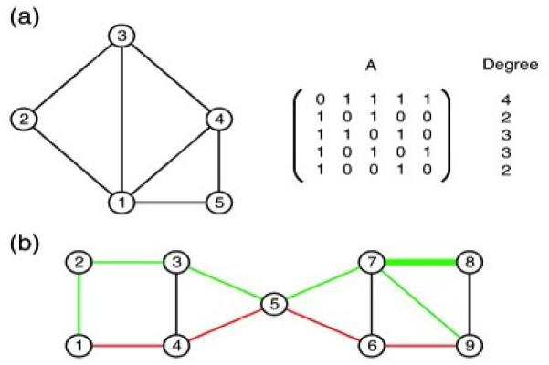
Schematic illustration of the graph theory concepts used in this paper. Figure (a) shows a simple, undirected graph with N = 5 nodes and 7 edges, along with the corresponding adjacency matrix, A. The degree of theith node can be obtained from the adjacency matrix simply by summing the entries in the ith row or column. In (b), we see an example of two different walks between nodes 1 and 9 of a network. The first walk 1  4
 5
 6
 9 (red), of length 4, gives the shortest walk between the two nodes. Whereas the second, longer walk 1
 2
 3
 5
 7
 8
 7
 9 (green) illustrates the fact that a walk may use the same link more thanonce; here the edge connecting nodes 7 and 8 is used twice in succession en route to node 9
Network communicability
Communication, to be understood here as transmission of information through a network, is usually considered to take place along geodesics. However, in many real-world networks the spread of information is not restricted only to shortest paths (Borgatti, 2005 and Newman, 2005); in the context of our study, a connection between two adjacent brain regions may be disrupted due to the stroke but the two regions may still be able to communicate via longer paths. Recently, Estrada and Hatano (2008) introduced the concept of communicability as a quantitative measure of the ease with which ‘information’ can spread across a network. This new measure deals with the issue that absence of an edge between a pair of nodes is not necessarily an indication of a low degree of ‘connectedness’ between them.
Estrada and Hatano assigned a measure of communicability between two nodes by counting the total number of walks between them, with walks of length k scaled by a factor of 1/ k !, so that longer walks have less influence than shorter walks. This scaling is particularly important in our context since experimental noise is expected to increase with walk length. In this way, communicability between distinct nodes i and j may be defined as (3)
which may be written
where exp denotes the matrix exponential.
In words, the communicability gives a weighted sum of the number of walks between nodes i and j; the weighting is such that shorter walks make a larger contribution. Weighted networks
In the present study, connectivity information, which is provided by the probabilistic tractography step, takes the from of real-valued, positive weights. Here a larger weight aij indicates a greater ‘strength’ of connection between nodes i and j (note that strength simply refers to the number of tractography streamlines that connect two nodes, and does not relate in a straightforward way to anatomical strength of connection). In this more general setting, both identities (1) and (2) remain valid, however, their interpretation changes slightly. In (1) the notion of degree is replaced by that of the weighted, or generalised, degree. Now, rather than counting the number of edges incident to node i we compute the sum of weights along incident edges. In the case of identity (2), rather than simply making a zero/one contribution depending upon whether the walk i  r1
 r2
 ⋯ rk − 1
 j is possible, the term ai, r1ar1, r2 … ark − 2, rk − 1ark − 1, j contributes the product of the weights along all the edges in the walk.
Although it is possible to define communicability for a weighted network as in Eq. (3), difficulties are likely to arise if the weights are poorly calibrated. Nodes with unusually large weights typically dominate the results. Crofts and Higham (2009) therefore argued for a normalisation step in which the weight aij is divided by the product
allowing communicability between distinct nodes i and j in a weighted network to be defined as (4)
Here the N × N diagonal matrix
The study in (Crofts and Higham, 2009) showed that this new measure adds significant value to the raw connectivity data when unsupervised classification methods are to be applied.
Note that the communicability matrix can be used to define a new network - the so called communicability network - whose nodes coincide with those of the original network, but whose weighted links are given by Eq. (4). In the analysis to follow the communicability network is used as the basis of our computational study.
Spectral clustering
In order to compare the two classes, strokes and controls, we build a new m × 27 (27 = 9 + 18 number of data sets) data matrix Adata, whose columns, (Adata)j, contain the m attributes of interest for the jth subject. For example, when we attempt to distinguish between the two classes by looking for changes in their respective connectivity patterns, we consider connections between every pair of brain regions and so we take as attributes the 1540 (= (562 – 56) /2) distinct connectivity weights—this matrix will be denoted Aconn. Another attribute that we compare between groups is the generalised degree. Now, the i, jth entry of the 56 × 27 data matrix, Adeg, contains the generalised degree of the ith node (brain region) for the jth subject. The generalised degree matrix carries less detailed information than the full connectivity matrix, Aconn, but it has the benefit of dealing directly with individual brain regions, as opposed to connections between brain regions, making classification results easier to interpret. Note that a similar construction can be performed for the communicability networks, and in this case we use Cconn and Cdeg to denote the respective data matrices. To summarise, matrices Aconn and Cconn represent the connectivity or communicability between all pairs of brain regions in each subject; Adeg and Cdeg summarise connectivity or communicability scores for each brain region in each subject. While connectivity scores reflect the direct path between two regions, communicability scores reflect direct and all possible indirect paths.
We perform unsupervised clustering of subjects based on connectivity data in order to assess how accurately we can distinguish between strokes and controls. Unsupervised clustering was performed using the singular value decomposition (SVD; Higham et al., 2007). The approach is closely related to many other techniques, such as Principal Components Analysis, support vector machines/kernel based methods, machine learning and multidimensional scaling (Cox & Cox, 1994, MacKay, 2003 and Skillicorn, 2007). It compresses large amounts of information into a small number of dimensions, allowing for simple visual interpretation of the data and for further processing, such as clustering or ranking.
In the case of compression to one dimension, the ith subject is represented by a single real number, given by the ith component of a right singular vector,v[2]. We focus here on the extent to which v[2] is able to differentiate between subject types. In the case where the 56 × 27 generalised degree matrix Cdeg is used, the corresponding left singular value, u[2], has 56 components and thereby assigns a number to each brain region. If v[2] successfully separates the two groups, then the extreme (most positive and most negative) components in u[2] indicate which brain regions are most responsible for the separation.
Statistical Validation
In order to determine which brain regions were driving any separation between groups we performed a repeated measures ANOVA on the communicability degree (Cdeg) scores for each region followed by post-hoc independent samples t-tests comparing Cdeg between patients and controls for each of the 56 brain regions considered. We used Bonferonni correction to calculate a t-threshold of t > 3.75 (df = 25) to be equivalent to a corrected probability threshold of p < 0.05 (uncorrected p = 0.05/56 = 0.0009). We also report trends at t > 3.4 (corrected p < 0.1, uncorrected p = 0.1/56 = 0.002). For regions found to have a significant change in Cdeg we tested for a change in Cconn for each connectionof each region using independent sample t-tests with a corrected t-threshold of t > 3.7(df = 25) and tested for correlations between Cdeg and Fugl-Meyer score, stroke volume and time post stroke using Pearson correlation and a Bonferroni corrected p-threshold of p = 0.05/ (number of regions tested).
Results
Spectral Clustering Using Connectivity and Communicability Measures
Measures of connectivity (‘direct’ connections) and communicability (direct plus indirect connections) between all network nodes were stored in matrices of 1540 values by 27 subjects (Aconn and Cconn). Matrices of measures of degree (Adeg and Cdeg) summarise connectivity or communicability measures for each of the 56 brain regions for each subject. We applied spectral clustering to Aconn, Cconn, Adeg and Cdeg (Fig. 2). Most measures broadly separated stroke patients from healthy control subjects. Interestingly, this separation was apparent not only using data from the lesioned (left) hemisphere but also based on data from the contralesional (right) hemisphere (Fig. 2). This clustering did not simply reflect gender differences (Supplementary Figure 5).
Fig. 2.
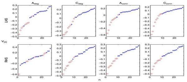
Comparison of both connectivity and communicability measures for left (top) and right (bottom) hemispheres. Ordered components of the second right singular vector v[2] of Adeg, Cdeg, Aconn and Cconn broadly separated strokes and controls in both left (lesioned) and right hemispheres. Circles denote stroke patients and crosses denote controls.
While it is unsurprising that structural connectivity is altered in the lesioned hemisphere, the observation that communicability of structural networks in the contralesional hemisphere also differentiates between groups merits further interrogation. We opted to explore this finding using the communicability measures (Cconn and Cdeg) as these performed better than connectivity measures (Aconn and Adeg) in separating patients from controls (Fig. 2). We first tested whether the separation was driven by particular brain regions or connections. While the total number of connections under consideration is large (1540), the number of brain regions (56) is more amenable to exploration. To limit the multiple comparisons problem, we chose first to test whether specific brain regions were implicated and then to test whether particular connections from those regions were involved. An inspection of the u[2] scores for both hemispheres reveals that extreme values from a small number of brain regions are driving the separation between patients and controls (Fig. 3).
Fig. 3.
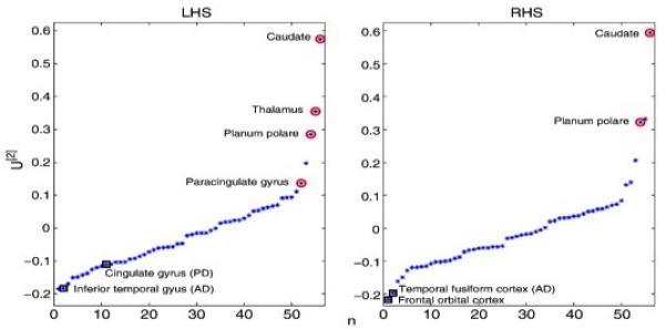
u[2] scores for each of the 56 brain regions considered for the left hemisphere (left) and right hemisphere (right). Extreme values of u[2] will drive the separation of individuals into classes. Note that we have enclosed those brain regions returned as significant by our statistical analysis and labelled them accordingly. Red circles denote those brain regions that were found to have diminished communicability scores in strokes, whilst black squares highlight regions showing a relative increase.
Between Group Differences in Communicability Measures
A repeated measures ANOVA of communicability degree scores for each of the 56 regions across both hemispheres revealed a highly significant effect of hemisphere (F(1, 25) = 9.5, p = 0.005) so we went on to test data from left (lesioned) and right (contralesional) hemisphere separately. A repeated measures ANOVA of data from the left (lesioned) hemisphere revealed a significant main effect of brain area (F(55, 1375) = 66.4, p < 0.001), a significant interaction between area and group (F(55, 1375) = 7.0, p < 0.001), and a trend towards a main effect of group (F(1, 25) = 3.5, p = 0.07). An analysis of data from the right (contralesional) hemisphere showed a significant main effect of area (F(55, 1375) = 66.0, p < 0.001) and a significant interaction between area and group (F(55, 1375) = 6.0, p < 0.01) but no main effect of group (F(1, 25) = 0.94, p = 0.3).
Location of Regions of Altered Communicability
Given the interactions with group identified by the ANOVAs, we performed a series of post-hoc t-tests to compare the communicability degree between patients and controls for each brain region separately (Fig. 4).
Fig. 4.
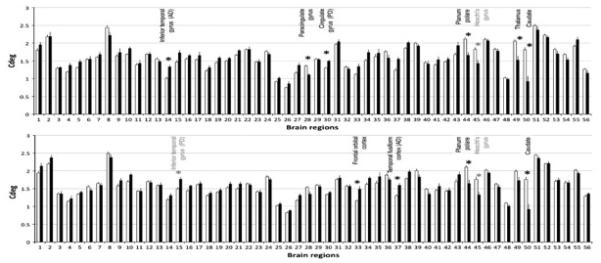
Mean communicability degree scores per brain region for the left (lesioned) hemisphere (top) and the right (contralesional) hemisphere (bottom). White bars show control and black bars show stroke data. Error bars are standard errors. Asterisks indicate significant differences between patients and controls, corrected for multiple comparisons, at corrected p < 0.05 (black asterisks) or trends (corrected p < 0.1, grey asterisks).
Stroke patients showed significantly reduced Cdeg (compared with healthy controls) in relation to left (lesioned) hemisphere regions including the caudate (t = 6.1, corrected p < 0.001), paracingulate gyrus (t = 5.1, df = 25, corrected p < 0.001), thalamus (t = 4.9, corrected p = 0.003), and planum polare (t = 4.7, corrected p = 0.005) and trends for reduced values in relation to Heschl’s gyrus (t = 3.7, corrected p = 0.06) (Fig. 4a). In the right (contralesional) hemisphere, stroke patients showed significantly reduced communicability compared with healthy controls in relation to the caudate (t = 5.7, corrected p < 0.001), and planum polare (t = 4.3, corrected p = 0.013) and trends for reduced values in relation to Heschl’s gyrus (t = 3.6, corrected p = 0.077) (Fig. 4b).
Patients showed significantly increased communicability degree compared with healthy controls in relation to left (lesioned) hemisphere regions including the inferior temporal gyrus (anterior division; t = – 4.6, corrected p = 0.006) and cingulate gyrus (posterior division) (t = – 4.4, p = 0.01) (Fig. 4a). In the right (contralesional) hemisphere, patients showed significantly increased Cdeg compared with healthy controls in relation to the orbitofrontal cortex (t = – 4.7, corrected p = 0.0045) and temporal fusiform cortex (anterior division; t = – 4.3, corrected p = 0.013) and a trend for higher values in relation to the inferior temporal gyrus (posterior division; t = – 3.6, corrected p = 0.077) (Fig. 4b).
For each region found to have altered communicability degree in patients, we went on to test for significant differences in communicability scores (Cconn) for individual connections between patients and controls (Supplementary Table 1). Amongst areas showing reduced Cdeg in patients compared with controls, significant reductions in Cconn were widespread (20/55 connections) for the caudate in the lesioned hemisphere. Other regions in the lesioned and contralesional showed a more selective pattern of significantly increased communicability over connections (left thalamus (8/56), left planum polare (5/55); left paracingulate (0/55); right caudate (7/55); right planum polare (6/55)). For regions in which we found increased Cdeg in patients compared with controls, significant increases in Cconn were found in very few connections for either hemisphere (Supplementary Table 2; left posterior cingulate (0/55); left inferior frontal gyrus, anterior division (4/55); right frontal orbital cortex (3/55); right temporal fusiform gyrus (1/55)).
In addition, for those regions showing a significant difference in Cdeg between patients and controls, we tested for correlations between Cdeg and Fugl-Meyer score, stroke volume and time post-stroke within the patient group. None of these correlations was significant (all corrected p > 0.05).
We went on to consider the spatial distribution of regions of altered communicability in patients relative to the location of stroke lesions. In this group of highly selected stroke patients, lesions were clustered around the internal capsule, basal ganglia region (Fig. 5). Regions of reduced communicability in stroke patients tended to be located around the lesion sites in the lesioned hemisphere and around their homologous locations in the contralesional hemisphere (Fig. 5). Regions of increased communicability in patients were located in prefrontal, cingulate and temporal cortical regions (Fig. 5). We have previously tested for differences in fractional anisotropy (FA) between the patients and control subjects studied here (Bosnell et al., submitted for publication) and have overlaid those findings onto the results reported here in Fig. 5. In the lesioned hemisphere, regions of reduced communicability co-localised with regions of reduced FA (Fig. 5). In the contralesional hemisphere, however, our previous study of FA only found evidence for reductions in some parts of the corpus callosum. We did not previously find evidence for reduced FA around the pathways showing reduced communicability in the contralesional hemisphere in the current study.
Fig. 5.
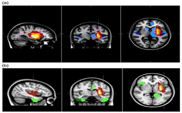
Spatial relationships between stroke lesions, regions associated with reduced communicability degree, and pathways showing reduced FA. Overlap map of stroke lesions is shown in red to white (where colorscale indicates number of patients in whom a lesion is present) in the region of the internal casule/basal ganglia of the left hemisphere. Top row also indicates grey matter regions of interest associated with reduced communicability in patients relative to controls (in blue, where light blue regions are significant (p < 0.05 corrected) and dark blue regions show trends (p < 0.1, corrected). These areas associated with reduced communicability tend to be located around the stroke lesions in the lesioned hemispheres and in homologues locations in the contralesional hemsiphere. Top row also shows narrow pink lines within the white matter that indicate regions of reduced FA on the white matter ‘skeleton’ detected in our previous study of FA in this population (Bosnell et al., submitted for publication). This shows that whereas FA reductions are widespread in the lesioned hemiphere, they are restricted to the corpus callosum of the contralesional hemisphere and do not appear around the regions associated with reduced communicability in this hemisphere. Bottom row indicates grey matter regions of interest associated with increased communicability in patients relative to controls (in green, where light green regions are significant (p < 0.05, corrected) and dark green region shows a trend (p < 0.1, corrected).
Basic Network Measures in Patients and Controls
To test whether the communicability measure provided information beyond that available from basic network measures we compared histograms of matrix norms, weighted clustering coefficients, and degree distributions, between patients and controls (Supplementary Figures 9, 10 and 11). None of these measures differentiated between patients and controls using data from the contralesional hemisphere. While these measures capture certain features of the network architecture, they do not appear to preserve information on the correspondence between nodes across subjects; such correspondences are important for capturing between-group differences. Spectral reordering based on weighted path-length, weighted clustering coefficients and eigenvector centrality also failed to differentiate between patients and controls (Supplementary Figures 12, 13 and 14).
Discussion
Using novel network analysis methods, we found evidence for altered structural connectivity not only in the lesioned hemisphere but also in the contralesional hemisphere of chronic stroke patients. Clustering of individuals according to measures of structural connectivity scores broadly separated patients with sub-cortical left hemisphere strokes from age-matched controls using data from the left (lesioned) hemisphere or the right (contralesional) hemisphere, particularly when both direct and indirect connections were considered by using a measure of “communicability”. This finding suggests that alterations in white matter structure that influence network measures of efficiency of communication are present in both hemispheres following stroke.
We found that the communicability scores of a few brain regions drove separation of patients and controls. Our highly selected patient group all had subcortical strokes located around the basal ganglia/internal capsule. Regions of reduced communicability in patients tended to cluster around the stroke locations: in the lesioned hemisphere these included the caudate, paracingulate gyrus, thalamus, planum polare and Heschl’s gyrus. A subset of these regions (caudate, planum polare, Heschl’s gyrus) also showed evidence for reduced communicability in patients in the contralesional hemisphere. These areas in the contralesional hemisphere are remote from the site of primary damage, but are anatomically connected, directly or indirectly, with their homologues in the lesioned hemisphere (Fisher et al., 1984 and Pandya & Rosene, 1993 ).
This pattern of reduced communicability shows some similarities to previously reported patterns of secondary degeneration detected using other imaging modalities or measures. For example, diffusion studies of fractional anisotropy (FA) reveal patterns of anterograde (Wallerian) and retrograde white matter tract degeneration in pathways in the lesioned hemisphere connected to a site of primary damage (Liang et al., 2007, Pierpaoli et al., 2001, Thomalla et al., 2004 and Werring et al., 2000). Although such changes are rarely detected in the contralesional hemisphere, observations of transhemispheric diaschisis (Andrews, 1991) support the idea that widespread interconnected regions, even in the contralesional hemisphere, can be functionally and structurally altered after a focal lesion. We propose that multivariate network measures such as that used here are more sensitive for detection of subtle transhemispheric connectivity change than the simple, univariate diffusion MRI measures of white matter structure.
In addition to regions of reduced communicability, we also found some areas of greater communicability in patients compared to controls: the left (lesioned) anterior inferior temporal gyrus and posterior cingulate gyrus and the right (contralesional) orbitofrontal cortex, anterior temporal fusiform cortex and posterior inferior temporal gyrus. One possible interpretation of these changes is that increased communicability reflects adaptive changes in white matter structure that have occurred secondary to the stroke. Consistent with this possibility, a previous study, using FA as a measure of white matter microstructure, reported increased FA in patients in an area of the corticospinal tract where a positive correlation between FA and motor skill was found (Schaechter et al., 2009) and animal studies have reported formation of novel cortico-cortical connections following damage (Dancause et al., 2005). Furthermore, longitudinal studies in healthy subjects support the idea that functionally significant white matter structural changes can occur over weeks or months in the adult human brain ( Keller & Just, 2009 and Scholz et al., 2009). An alternative hypothesis is that the changes predated the lesion and represent a marker of stroke risk. However, apparent increases in connectivity measures when using probabilistic tractography also could be an indirect consequence of decreases of tract integrity elsewhere. This possibility arises because a fixed number of tractography streamlines are initiated from each seed voxel. Therefore, if the connectivity of some regions is reduced, then the pathways that should have reached those regions must have either reached other targets or been terminated for other reasons (in practice exceeding the curvature threshold). Increased uncertainty on estimates of fiber directions (due to the presence of white matter damage) will result in tractography pathways diverging away from their true destination and potentially accumulating in adjacent regions. However, pathways relating to the specific regions associated with increased communicability in the current study do not have an obvious anatomical relationship to those damaged by the stroke. It is therefore difficult to interpret the increased communicability finding with confidence. Future longitudinal studies, using network measures of brain structure, could be used to distinguish hypotheses concerning risk-related, adaptive, or incidental change related to focal damage.
The current study is limited by the small number of patients tested. However, our patient group was highly selected to include only those with left hemisphere subcortical stroke. Enforcing strict anatomical inclusion criteria means that relatively consistent regional responses were expected, increasing study sensitivity. It is well established that age has significant effects on anatomical connectivity, with increasing age associated with decreasing microstructural integrity (Giorgio et al., 2010, Pfefferbaum et al., 2000 and Salat et al., 2005) and decreased probability of anatomical connectivity between cortical regions (Gong et al., 2009). We selected healthy controls that were age-matched to our stroke group, but both groups had a wide age range. We demonstrated, however, that age did not have any effect on our clustering of individuals into groups (Supplementary Figure 6) and so we do not believe that the wide age range influenced the results of interest.
In mathematical terms, communicability assesses the ease with which information can flow across a network (Crofts & Higham, 2009 and Estrada & Hatano, 2008) using both direct and indirect routes between nodes, but interpretation of this measure in biological terms is challenging. Our data only reflect structural properties of the white matter and so we have no assessment of information flow in a physiological sense. The structure of the network that we construct depends on the connectivity values provided by diffusion tractography and will therefore reflect the integrity of white matter connections between brain regions. Communicability assesses how easy it is to travel between nodes in the constructed network and will therefore depend in part on the structural integrity of pathways. However, it is important to note that the effects detected in our current study have not been observed in previous studies using more conventional measures of white matter microstructure, such as FA: our prior study of this same cohort did not detect extensive reductions in FA in the contralesional hemisphere using whole brain analysis (Bosnell et al., submitted for publication), consistent with a previous region-of-interest study of FA changes following stroke (Liang et al., 2007). Therefore, the weighted communicability measure may offer increased sensitivity to subtle change in brain structural networks, particularly if the precise location of change is difficult to predict.
Brain network analysis has been shown to depend on the strategy used for brain parcellation and node definition (Wang et al., 2009 and Zalesky et al., 2010). Here, we used an atlas of cortical regions to define nodes. It is possible that greater sensitivity could be achieved by using individually defined cortical parcellations, based on gross anatomical landmarks or on the connectivity data themselves (Perrin et al., 2008).
Our results highlight the possibilities offered by network characterisation of brain structure in disease and complement recent studies using connectivity analyses to interrogate functional network changes after stroke ( Grefkes et al., 2008, Mintzopoulos et al., 2009 and Sharma et al., 2009). Functional studies have found, for example, that even when regional activation patterns and motor behaviour appear normal in patients, there is evidence for reduced functional connectivity between premotor and supplementary areas duringmovement (Sharma et al., 2009). Future studies should exploit the power of network analysis of brain structure and function to gain a fuller understanding of the processes of degeneration or adaptation that occur following stroke.
Supplementary Material
References
- Andrews RJ. Transhemispheric diachisis. A review and comment. Stroke. 1991;22(7):943–949. doi: 10.1161/01.str.22.7.943. [DOI] [PubMed] [Google Scholar]
- Barabasi AL. Scale-free networks: a decade and beyond. Science. 2009;325(5939):412–413. doi: 10.1126/science.1173299. [DOI] [PubMed] [Google Scholar]
- Basser PJ, Mattiello J, LeBihan D. MR diffusion tensor spectroscopy and imaging. Biophys. J. 1994;66(1):259–267. doi: 10.1016/S0006-3495(94)80775-1. [DOI] [PMC free article] [PubMed] [Google Scholar]
- Bassett D, Bulmore E, Verchinski BA, Mattay VS, Weinberger DR, Meyer-Lindenberg A. Hierarchical organization of human cortical networks in health and schizophrenia. J. Neurosci. 2008;28(37):9239–9248. doi: 10.1523/JNEUROSCI.1929-08.2008. [DOI] [PMC free article] [PubMed] [Google Scholar]
- Beaulieu C. The basis of anisotropic water diffusion in the nervous system - a technical review. NMR Biomed. 2002;15(7–8):435–455. doi: 10.1002/nbm.782. [DOI] [PubMed] [Google Scholar]
- Beaulieu C. The biological basis of diffusion anisotropy. In: Johansen-Berg H, Behrens TEJ, editors. Diffusion MRI: From quantitative measurement to in-vivo neuroanatomy. Elsevier; London: 2009. [Google Scholar]
- Behrens TEJ, Woolrich MW, Jenkinson M, Johansen-Berg H, Nunes RG, Clare S, Matthews PM, Brady JM, Smith SM. Characterization and propagation of uncertainty in diffusion-weighted MR imaging. Magn. Reson. Med. 2003;50(5):1077–1088. doi: 10.1002/mrm.10609. [DOI] [PubMed] [Google Scholar]
- Behrens TEJ, Jbabdi S, Woolrich MW, Andersson JL. A Bayesian framework for global tractography. Neuroimage. 2007;37(1):116–129. doi: 10.1016/j.neuroimage.2007.04.039. [DOI] [PubMed] [Google Scholar]
- Biernaskie J, Corbett D. Enriched rehabilitative training promotes improved forelimb motor function and enhanced dendritic growth after focal ischemic injury. J. Neurosci. 2001;21(14):5272–5280. doi: 10.1523/JNEUROSCI.21-14-05272.2001. [DOI] [PMC free article] [PubMed] [Google Scholar]
- Borgatti SP. Centrality and network flow. Soc. Networks. 2005;27:55–71. [Google Scholar]
- Bosnell R, Stagg C, Kincses ZT, Kischka U, Matthews PM, Johansen-berg H. Contralesional white matter microstructure integrity contributes to determining new motor skill learning after stroke. submitted for publication.
- Bullmore E, Sporns O. Complex brain networks: graph theoretical analysis of structural and functional systems. Nat. Neurosci. Rev. 2009;10:186–198. doi: 10.1038/nrn2575. [DOI] [PubMed] [Google Scholar]
- Cox TF, Cox MAA. Multidimensional Scaling. Chapman and Hall; London: 1994. [Google Scholar]
- Crofts JJ, Higham DJ. A weighted communicability measure applied to complex brain networks. J. R. Soc. Interface. 2009;6(33):411–414. doi: 10.1098/rsif.2008.0484. [DOI] [PMC free article] [PubMed] [Google Scholar]
- Dancause N, Barbay S, Frost SB, Plautz EJ, Chen D, Zoubina EV. Extensive cortical rewiring after brain injury. J. Neurosci. 2005;25(44):10167–10179. doi: 10.1523/JNEUROSCI.3256-05.2005. [DOI] [PMC free article] [PubMed] [Google Scholar]
- Estrada E, Hatano N. Communicability in complex networks. Phys. Rev. E. 2008;77:036111. doi: 10.1103/PhysRevE.77.036111. [DOI] [PubMed] [Google Scholar]
- Fisher RS, Shiota C, Levine MS, Hull CD, Buchwald NA. Interhemispheric organization of corticocaudate projections in the cat: a retrograde double-labelling study. Neurosci. Lett. 1984;1(25–30) doi: 10.1016/0304-3940(84)90066-1. [DOI] [PubMed] [Google Scholar]
- Giorgio A, Santelli L, Tomassini V, Bosnell R, Smith S, Stefano ND. Age-related changes in grey and white matter structure throughout adulthood. Neuroimage. 2010;51(3):943–951. doi: 10.1016/j.neuroimage.2010.03.004. [DOI] [PMC free article] [PubMed] [Google Scholar]
- Gong G, Rosa-Neto P, Carbonell F, Chen ZJ, He Y, Evans AC. Age- and gender-related differences in the cortical anatomical networks in the human brain. J. Neurosci. 2009;29(50):15684–15693. doi: 10.1523/JNEUROSCI.2308-09.2009. [DOI] [PMC free article] [PubMed] [Google Scholar]
- Grefkes C, Nowak DA, Eickhoff SB, Dafotakis M, Kust J, Karbe H. Cortical connectivity after subcortical stroke assessed with functional magnetic resonance imaging. Ann. Neurol. 2008;63(2):236–246. doi: 10.1002/ana.21228. [DOI] [PubMed] [Google Scholar]
- He Y, Chen ZJ, Evans A. Small-world anatomical networks in the human brain revealed by cortical thickness from MRI. Cereb. Cortex. 2007;17:2407–2419. doi: 10.1093/cercor/bhl149. [DOI] [PubMed] [Google Scholar]
- He Y, Chen Z, Evans A. Structural insights into aberrant topolgical patterns of large-scale cortical networks in Alzheimer’s disease. J. Neurosci. 2008;28(18):4756–4766. doi: 10.1523/JNEUROSCI.0141-08.2008. [DOI] [PMC free article] [PubMed] [Google Scholar]
- Higham DJ, Kalna G, Kibble M. Spectral clustering and its use in bioinformatics. J. Comput. Appl. Math. 2007;204:25–37. [Google Scholar]
- Iturria-Medina Y, Sotero RC, Canales-Rodriguez EJ, Alemán-Gómez Y, Melie-Garcia L. Studying the human brain anatomical network via diffusion weighted MRI and Graph Theory. Neuroimage. 2008;40:1064–1076. doi: 10.1016/j.neuroimage.2007.10.060. [DOI] [PubMed] [Google Scholar]
- Johansen-Berg H, Rushworth MF, Bogdanovic MD, Kischka U, Wimalaratna S, Matthews PM. The role of ipsilateral premotor cortex in hand movement after stroke. Proc. Natl. Acad. Sci. 2002;99(22):14518–14523. doi: 10.1073/pnas.222536799. [DOI] [PMC free article] [PubMed] [Google Scholar]
- Jones TA, Kleim JA, Greenough WT. Synaptogenesis and dendritic growth in the cortex opposite unilateral sensorimotor cortex damage in adult rats: a quantitative electron microscopic examination. Brain Res. 1996;733(1):142–148. doi: 10.1016/0006-8993(96)00792-5. [DOI] [PubMed] [Google Scholar]
- Jones DK, Simmons A, Williams SC, Horse field MA. Non-invasive assessment of axonal fiber connectivity in the human brain via diffusion tensor MRI. Magn. Reson. Med. 1999;42(1):37–41. doi: 10.1002/(sici)1522-2594(199907)42:1<37::aid-mrm7>3.0.co;2-o. [DOI] [PubMed] [Google Scholar]
- Keller TA, Just MA. Altering cortical connectivity: remediation-induced changes in the white matter of poor readers. Neuron. 2009;64(5):624–631. doi: 10.1016/j.neuron.2009.10.018. [DOI] [PMC free article] [PubMed] [Google Scholar]
- Liang Z, Zeng J, Liu S, Ling X, Xu A, Yu J. A prospective study of secondary degeneration following subcortical infarction using diffusion tensor imaging. J. Neurol. Neurosurg. Psychiatry. 2007;78(6):581–586. doi: 10.1136/jnnp.2006.099077. [DOI] [PMC free article] [PubMed] [Google Scholar]
- Lotze M, Markert J, Hoppe PSJ, Plewnia C, Gerloff C. The role of multiple contralesional motor areas for complex hand movements after internal capsular lesion. J. Neurosci. 2006;26(22):6096–6102. doi: 10.1523/JNEUROSCI.4564-05.2006. [DOI] [PMC free article] [PubMed] [Google Scholar]
- MacKay DJC. Information Theory, Inference and Learning Algorithms. Cambridge University Press; Cambridge: 2003. [Google Scholar]
- Mintzopoulos D, Astrakas LG, Khanicheh A, Konstas AA, Singhal A, Moskowitz MA, Rosen BR, Tzika AA. Connectivity alterations assessed by combining FMRI and MR-compatible hand robots in chronic stroke. Neuroimage. 2009;47(S2):T90–T97. doi: 10.1016/j.neuroimage.2009.03.007. [DOI] [PMC free article] [PubMed] [Google Scholar]
- Mori S, Crain BJ, Chacko VP, van Zijl PC. Three-dimensional tracking of axonal projections in the brain by magnetic resonance imaging. Ann. Neurol. 1999;45(2):265–269. doi: 10.1002/1531-8249(199902)45:2<265::aid-ana21>3.0.co;2-3. [DOI] [PubMed] [Google Scholar]
- Newman MEJ. A measure of betweeness centrality based on random walks. Soc. Networks. 2005;27:39–54. [Google Scholar]
- Pandya DN, Rosene DL. Laminar termination patterns of thalamic, callosal, and association afferents in the primary auditory area of the rhesus monkey. Exp. Neurol. 1993;119(2):220–234. doi: 10.1006/exnr.1993.1024. [DOI] [PubMed] [Google Scholar]
- Perrin M, Cointepas Y, Cachia A, Poupon C, Thirion B, Riviere D. Connectivity based parcellation of the cortical mantle using q-ball diffusion imaging. Int. J. Biomed. Imaging. 2008;2008:368–406. doi: 10.1155/2008/368406. [DOI] [PMC free article] [PubMed] [Google Scholar]
- Pfefferbaum A, Sullivan EV, Hedehus M, Lim KO, Adalsteinsson E, Moseley M. Age-related decline in brain white matter anisotropy measured with spatially corrected echo-planar diffusion tensor imaging. Magn. Reson. Med. 2000;44(2):259–268. doi: 10.1002/1522-2594(200008)44:2<259::aid-mrm13>3.0.co;2-6. [DOI] [PubMed] [Google Scholar]
- Pierpaoli C, Barnett A, Pajevic S, Chen R, Penix LR, Virta A. Water diffusion changes in Wallerian degeneration and their dependence on white matter architecture. Neuroimage. 2001;13(6):1174–1185. doi: 10.1006/nimg.2001.0765. [DOI] [PubMed] [Google Scholar]
- Salat DH, Tuch DS, Greve DN, van der Kouwe AJ, Hevelone ND, Zaleta AK. Age-related alterations in white matter microstructure measured by diffusion tensor imaging. Neurobiol. Aging. 2005;15(9):1332–1342. doi: 10.1016/j.neurobiolaging.2004.09.017. [DOI] [PubMed] [Google Scholar]
- Salvador R, Suckling J, Schwarzbauer C, Bullmore E. Neurophysiological architecture of functional magnetic resonance images of the human brain. Cereb. Cortex. 2005;15:1332–1342. doi: 10.1093/cercor/bhi016. [DOI] [PubMed] [Google Scholar]
- Schaechter JD, Fricker ZP, Perdue KL, Helmer KG, Vangel MG, Greve DN. Microstructural status of ipsilesional and contralesional corticospinal tract correlates with motor skill in chronic stroke patients. Hum. Brain Mapp. 2009;30(11):3461–3474. doi: 10.1002/hbm.20770. [DOI] [PMC free article] [PubMed] [Google Scholar]
- Scholz J, Klein MC, Behrens TE, Johansen-berg H. Training induces changes in white-matter architecture. Nat. Neurosci. 2009;12(11):1370–1371. doi: 10.1038/nn.2412. [DOI] [PMC free article] [PubMed] [Google Scholar]
- Sharma N, Baron JC, Rowe JB. Motor imagery after stroke: relating outcome to motor network connectivity. Ann. Neurol. 2009;66(5):604–616. doi: 10.1002/ana.21810. [DOI] [PMC free article] [PubMed] [Google Scholar]
- Skillicorn D. Understanding Complex Datasets. Chapman & Hall/CRC; 2007. [Google Scholar]
- Smith SM, Jenkinson M, Woolrich MW, Beckmann CF, Behrens TEJ, Johansen-Berg H, Bannister PR, Luca MD, Drobnjak I, Flitney DE, Niazy RK, Saunders J, Vickers J, Zhang Y, Stefano ND, Brady MJ, Matthews PM. Advances in functional and structural MR image analysis and implementation as FSL. Neuroimage. 2004;23(S1):208–219. doi: 10.1016/j.neuroimage.2004.07.051. [DOI] [PubMed] [Google Scholar]
- Thomalla G, Glauche V, Koch MA, Beaulieu C, Weiller C, Rother J. Diffusion tensor imaging detects early Wallerian degeneration of the pyramidal tract after ischemic stroke. Neuroimage. 2004;22(4):1767–1774. doi: 10.1016/j.neuroimage.2004.03.041. [DOI] [PubMed] [Google Scholar]
- Wang J, Wang L, Zang Y, Yang H, Gong Q. Parcellation-dependent small-world functional networks: a resting state FMRI study. Hum. Brain Mapp. 2009;30(5):1511–1523. doi: 10.1002/hbm.20623. [DOI] [PMC free article] [PubMed] [Google Scholar]
- Werring DJ, Toosy AT, Clark CA, Parker GJ, Barker GJ, Miller DH. Diffusion tensor imaging can detect and quantify corticospinal tract degeneration after stroke. J. Neurol. Neurosurg. Psychiatry. 2000;69(2):269–272. doi: 10.1136/jnnp.69.2.269. [DOI] [PMC free article] [PubMed] [Google Scholar]
- Zalesky A, Fornito A, Harding IH, Cocchi L, Yucel M, Pantelis C. Whole-brain anatomical networks: does the choice of nodes matter? Neuroimage. 2010;50(3):970–983. doi: 10.1016/j.neuroimage.2009.12.027. [DOI] [PubMed] [Google Scholar]
Associated Data
This section collects any data citations, data availability statements, or supplementary materials included in this article.