


FIG. 2.
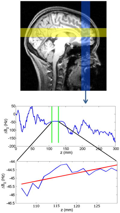
Top: 2-dimensional RF pulses sequentially excite three spatial columns, two of which are shown in yellow and blue on a sagittal brain cross section (the third column is perpendicular to the page). Two gradient echoes are acquired for each column. Center: a phase difference map for the inferior-to-superior column, from which the B0 field distribution is calculated (averaged across the column cross-section). The values that fall inside the VOI (between green lines) are selected for further processing. Bottom: A linear fit is performed on ΔB0 values within the VOI (red line). The slope of this line provides one of the 3 components of the desired correction gradient.