



Abstract
Diffusion tensor imaging (DTI) is used to study tissue composition and architecture in vivo. To increase the signal to noise ratio (SNR) of DTI contrasts, studies typically use more than the minimum of 6 diffusion weighting (DW) directions or acquire repeated observations of the same set of DW directions. Simulation-based studies have sought to optimize DTI acquisitions and suggest that increasing the directional resolution of a DTI dataset (i.e., the number of distinct directions) is preferable to repeating observations, in an equal scan time comparison. However, it is not always clear how to translate these recommendations into practice when considering physiological noise and scanner stability. Furthermore, the effect of different DW schemes on in vivo DTI findings is not fully understood. This study characterizes how the makeup of a DW scheme, in terms of the number of directions, impacts the precision and accuracy of in vivo fractional anisotropy (FA), mean diffusivity (MD), and principal eigenvector (PEV) findings. Orientation dependence of DTI reliability is demonstrated in vivo and a principled theoretical framework is provided to support and interpret findings with simulation results. As long as sampling orientations are well balanced, differences in DTI contrasts due to different DW schemes are shown to be small relative to intra-session variability. These differences are accentuated at low SNR, while minimized at high SNR. This result suggests that typical clinical studies, which use similar protocols but different well-balanced DW schemes, are readily comparable within the experimental precision.
Introduction
Diffusion tensor imaging (DTI) is a magnetic resonance (MR) imaging technique that is sensitive to the random thermal motions of water and can provide contrasts which give insight about tissue architecture. A diffusion tensor is a simple, yet powerful, mathematical description of the underlying, three-dimensional diffusion process that can be estimated from a series of diffusion-weighted (DW) MR images (Basser et al., 1994). Typically, a DW image is created by applying a pair of magnetic field gradients (so-called dephasing and rephasing gradients) along a distinct direction in 3D space. The resulting image, therefore, shows signal attenuation in the direction of the applied gradient, and the degree of signal attenuation is proportional to the water diffusivity. A diffusion tensor may be estimated from as few as 6 DW images acquired along non-collinear directions and 1 minimally weighted () image. However, to increase the signal-to-noise ratio (SNR), more than 6 DW images are commonly acquired along 6 or more non-collinear directions. In the latter case there are two options: either to add additional DW directions or repeat existing DW directions. For example, if time permits the acquisition of 12 DW images in total, one can increase the directional resolution (DW images in 12 distinct directions) or increase the number of scan repetitions (2 repetitions of DW images in 6 distinct directions); both of which take the same amount of time.
A source of confusion may be how to properly interpret the literature when selecting a DW scheme. Substantial theoretical and experimental work has gone into developing optimized DW schemes (Alexander and Barker, 2005; Conturo et al., 1996; Hasan et al., 2001; Jones, 2004; Jones et al., 1999; Skare et al., 2000) that permit accurate and precise calculation of a diffusion tensor and diffusion tensor-derived contrasts (such as fractional anisotropy, mean diffusivity, etc.) which result from the tensor formalism (Batchelor et al., 2003; Hasan et al., 2004; Jones, 2003; Jones and Basser, 2004). Several commonly used DW schemes have emerged through research addressing different constraints and imaging objectives. For example, 6 DW direction schemes can be constructed with tetrahedral distributions (Conturo et al., 1996) that provide simple geometric sampling or dual gradient methods (Pierpaoli et al., 1996) that maximize gradient power, thereby achieving a shorter echo time (TE). When additional DW directions are desired, potential energy (PE) minimization methods (Jones et al., 1999) have been shown to ensure regular sampling and minimize the rotational dependence of noise propagation (Batchelor et al., 2003; Jones, 2004). It is important to note that when the number of directions in a DW scheme corresponds to a member of an icosahedral group (e.g., 6, 10, 15, 31), the minimized PE solution can be expressed analytically as the vertices of the corresponding polyhedron (Batchelor et al., 2003; Hasan et al., 2004). The diversity of available DW schemes is also increased by schemes with more than 6 directions that maximize gradient power at the expense of less evenly spaced sampling (Jones, 2004; Muthupallai et al., 1999).
Moreover, practical constraints, such as available scan time, propensity for data corruption due to patient motion, gradient hardware performance, and manufacturer software limitations, often dominate the decision regarding which set of DW directions is optimal for use in a DTI experiment. However, the use of different DW schemes may lead to different computed tensors, and ultimately inconsistencies in the derived contrasts. The effects of relevant DW schemes on the accuracy and precision of tensor estimations and the derived contrasts have been investigated by simulation (Jones, 2004; Skare et al., 2000) and with in vivo data (Jones, 2003; Ni et al., 2006; Skare et al., 2000). There is strong simulation evidence that increasing the directional resolution is preferable to increased scan repetitions in an equal scan time comparison with a decreasing effect size as the number of DW directions increases (Hasan et al., 2001; Jones, 2003, 2004; Jones et al., 1999; Papadakis et al., 1999; Skare et al., 2000).
In this study, we investigate how the number of directions, in a well-balanced DW scheme, affects DTI-derived contrasts through direct in vivo analyses of experimental data. This methodology exposes the potential impacts of real world factors including subject motion and imaging artifacts/distortion. In addition to the in vivo experiments, simulations were performed to understand the characteristics of the experimental data (e.g., experimental data used as a basis for simulation with modeled noise). With this approach, we investigate the explanatory power of the single tensor model and interpret the experimental results in the context of the simulation literature.
Ultimately, this study addresses the differential hypothesis that either (1) the theoretical estimation benefits of using 30 DW directions as opposed to five repeats of 6 DW directions are realized in practice, or (2) other intra-session and inter-session factors, such as physiological noise, registration accuracy, distortion artifacts, or gradient performance, dominate the accuracy of DW experiments so that the choice of the direction scheme is non-significant in practice. Stated simply, this study addresses a fundamental question: given a certain amount of time for a DTI study, which DW scheme should be used for optimally precise and accurate DTI-derived contrasts, and why? This is an important question to consider when designing experiments and comparing data from different institutions but remains largely unanswered. Furthermore, a principled theoretical framework is provided to support and interpret experimental findings relative to simulation results.
The specific objective of the present study was to characterize how the choice of DW scheme impacts the precision and accuracy of fractional anisotropy (FA), mean diffusivity (MD), and the principal eigenvector (PEV) based on in vivo experimental data, with simulations to clarify and interpret these results. We present methods to partition a general, high directional resolution DTI dataset into subsets with a lower directional resolution. Without these partition techniques, a substantially larger dataset would be required to investigate the differences due to different DW schemes. This study is a part of the Biomedical Informatics Research Network (BIRN) studies. Acquired and processed DTI data as well as the acquisition protocol for this study are freely available through the BIRN website (http://www.nbirn.net/Resources/Downloads/) and can be used as a data resource and reference for 1.5T scanners.
Methods
Data acquisition
A healthy 24-year-old male volunteer participated in this study. Local institutional review board approval and written informed consent were obtained prior to examination. All data were acquired using a 1.5T MR scanner (Intera, Philips Medical Systems, Best, The Netherlands) with body coil excitation and a six-channel phased array SENSE head coil for reception. Three scanning sessions were performed over 2 days with the subject repositioned between each session. In each scanning session, 15 DTI datasets were acquired, yielding a total of 45 DTI scans. Each DTI dataset was acquired with the following imaging protocol. A multi-slice, single-shot EPI (SENSE factor = 2.0), spin echo sequence (TR/TE= 3632/100 ms) was used to obtain 25 transverse slices parallel to the line connecting the anterior and posterior commissures with no slice gap and 2.5 mm nominal isotropic resolution (FOV= 240 × 240, data matrix= 96 × 96, zero-filled and reconstructed to 256 × 256). Diffusion weighting was applied along 30 distinct directions (Jones et al., 1999; Skare et al., 2000) with a gradient strength of G = 19.5 mT/m and a b-factor of 1000 s/mm2. Five minimally weighted images () were acquired and averaged on the scanner as part of each DTI dataset. The total scan time to acquire one DTI dataset (30 DW images and 5 images) was 2 min 18 s. The total time, including image reconstruction, to acquire 15 DTI datasets and one anatomical MRI in a scan session was approximately 45 min.
Motion correction and SNR calculations
DTI datasets were processed offline using Matlab (Mathworks, Natick, MA) routines running on a Sun Fire V880 server (Sun Microsystems, Mountain View, CA). All data were coregistered with a purpose-constructed method (Landman et al., 2006) utilizing FLIRT (FMRIBTs Linear Image Registration Tool, Oxford, UK) (Jenkinson et al., 2002) to remove rigid body motion with six degrees of freedom registration. The gradient tables, which specify the direction of the magnetic field gradient corresponding to each particular DWI, were corrected to compensate for the rotational component of the coregistration procedure. Diffusion tensors were calculated using a multivariate log-linear fitting method in which each DW image and its corresponding vector from the gradient table entered the diffusion tensor calculation as unique entries—i.e., no averaging of DW images was performed. These analysis methods were encapsulated and publicly released in CATNAP (Coregistration, Adjustment and Tensor-solving, a Nicely Automated Program, http://iacl.ece.jhu.edu/~bennett/catnap/, Johns Hopkins University School of Medicine, Baltimore, Maryland, USA).
The log-linear fit was performed with no restrictions on the sign of the eigenvalues. To prevent taking the log of zero, a voxel with an intensity of zero in a DW image was set to half of the smallest non-zero voxel intensity recorded. The eigenvector associated with the largest eigenvalue (), i.e., the principal eigenvector (PEV), is taken to represent the predominant fiber orientation in each voxel. In the color-coded PEV maps, the dominant fiber orientation in a voxel was represented by red, green, and blue colors which were assigned to right–left, anterior–posterior, and superior–inferior orientations, respectively (Jones et al., 1997; Pierpaoli, 1997).
There are several difficulties in calculating an experimental SNR value that can be precisely compared with the values resulting from simulation studies. Whereas the noise in simulation studies is a modeled parameter, the SNR in in vivo imaging is spatially varying (due to coil sensitivity) and is tissue dependent (via the interaction of imaging sequence parameters and local tissue characteristics, e.g., T1, T2, PD). Furthermore, MR images can be subject to chemical shift artifacts as well as artifacts due to field inhomogeneity, eddy currents, and EPI-based geometric distortions.
To compare results with the literature and ensure that subsequent simulation studies correspond to approximately the same SNR range as the experimental data, we used a manual region of interest calculation. For clarity, we report SNR in terms of power decibels and contrast ratio . The SNR in the splenium of the corpus callosum was approximately 25 dB (17.8:1) in the averaged image, which would indicate an approximate SNR of 18 dB (7.9:1) in a single image.
Partitioning and grouping of diffusion-weighted data
The DW data in this study were acquired with a PE optimized 30 direction scheme (Jones et al., 1999; Skare et al., 2000), hereafter referred to as the Jones30. To investigate the effects of different DW schemes, the Jones30 scheme was partitioned into optimal PE-minimized subsets of 6, 10, and 15 DW directions with a Monte Carlo pair-wise relaxation method (Landman et al., 2006). These subsets are denoted as PE6, PE10, and PE15, respectively. The objective in this optimization step was to identify the closest approximation of a minimum PE scheme possible given the limitation of using data acquired with the Jones30 DW scheme. The Appendix Table A1 tabulates which directions from the Jones30 scheme were assigned to each of the optimized PE schemes.
The selection of optimal subsets was accomplished by Monte Carlo restarting of a local gradient descent algorithm. The algorithm was initialized by selecting N directions at random from the Jones30 scheme. This subset of size N was then optimized through an exhaustive search that involved a member–non-member exchange to minimize the previously described PE function (Jones et al., 1999). Fig. 1A illustrates the DW directions obtained by optimization for the PE6, PE10, and PE15 schemes as compared to the standard Jones30. The PE of the partitioned DW schemes (99.0, 303.5, 726.7) was at most 1% higher than the unconstrained PE optima for the equivalent number of directions (98.3, 301.8, 719.5).
Fig. 1.

Minimum potential energy (PE) partitions of the Jones30 DW scheme. The optimal PE partitions (left) are evenly distributed as indicated by the shading which is proportional to the area of the spherical Voronoi tessellations of the DW directions. The realized directions are distinct (right) from the specified ones (left) because the gradient tables are corrected for subject motion. The right panel shows 30 clusters, where each cluster represents a specified DW direction and consists of three sub-clusters which represent realized DW directions from each session. The separation of the sub-clusters shows the inter-session effects, while the distribution of the symbols shows the intra-session effects. Large ovals indicate the subset of the Jones30 that was used to construct the PE6 partition.
It is important to note the differences between the specified DW direction and the realized diffusion weighting direction due to patient motion. We use the term “specified” to refer to the set of DW directions that are given to the MR scanner at the time of acquisition. These directions are relative to either the slice layout (e.g., measurement, phase, and slice orientations) which was the case for this study or the fixed magnetic coordinate frame (e.g., the bore), depending on the scanner settings. When a heterogeneous sample, e.g., a human brain, is placed in the scanner, the diffusion weighting is also relative to the position and orientation of the anatomy. It is possible that volunteers will move or rotate during a sequence, and therefore the relative orientation between the scanner coordinate system and the anatomy changes. Image coregistration corrects for this in that it forces voxels in one anatomical location of one scan to correspond to the same anatomical location in a subsequent scan. However, motion correction also changes the relationship between the anatomical and scanner coordinate systems, and thus the diffusion weighting. When rotating the anatomy to establish spatial correspondence, the DW direction in the gradient table must also be rotated so that the vector that describes the diffusion weighting is correctly interpreted relative to the anatomy. We refer to the corrected DW directions, which are slightly different than the “specified” ones, as the “realized” DW directions. In an ongoing retrospective analysis of patient motion of 160 DTI scans from 52 subjects (30 ataxic patients, 22 controls), we observed an average of 1.9 ± 0.87 mm of translation and 0.53 ± 0.38° of rotation over a 3 min 57s time period (results presented in poster format Landman et al., 2006). Even with a healthy, well-behaved subject in this study, the specified and realized DW directions were different by 0.20 ± 0.07° within each session and a much larger difference occurred between sessions due to subject positioning (Fig. 1B).
To provide a benchmark for the differences between “poor” and “good” DW schemes, a direction-wise closest approximation to the tetrahedral 6 scheme was generated from the 30 direction PE scheme, denoted Tetra6. The Appendix Table A2 lists the DW directions from the Jones30 scheme that were assigned to the Tetra6 scheme. This scheme has been shown to have a high condition number (a measure of noise propagation in the estimation process), produce DTI results that exhibit prominent dependence on orientation, and lead to low SNR results (Skare et al., 2000).
To test if the partitioned subsets were a good approximation of the unconstrained optimal PE schemes with an equivalent number of directions, Monte Carlo simulation experiments were performed on diffusion tensor data derived from in vivo human brain observations. To minimize arbitrary effects of orientation, the unconstrained optimal PE schemes were first reoriented so that the directions were most similar (under mean squared error) to those of the partitioned subsets. One thousand tensors with FA> 0.25 were randomly selected from the DTI results of an in vivo human brain experiment. For each tensor, 100 simulated observations were created by applying the tensor model of diffusion to the set of DW directions for each DW scheme (Stejskal and Tanner, 1965). Gaussian noise was added in quadrature (e.g., in the frequency domain) to the DWIs and so that the resulting images had a SNR of 20 dB (10:1), which is approximately equivalent to the SNR observed in the experimental data. Diffusion tensors were then estimated from the simulated data for the partitioned subsets and unconstrained optimized schemes, respectively. Comparison of the mean FA and PEV using each DW scheme revealed mean differences between the unconstrained optimal PE schemes and the optimal PE partition schemes of (1) less than 0.005 in FA and (2) less than 0.5° in PEV orientation, which are both less than the differences observed in repeated acquisitions using a 30 direction DW scheme (Farrell et al., 2006). Thus, the optimal subsets (PE6, PE10, PE15) are deemed appropriate surrogates for the unconstrained optimal schemes.
To ensure a scan time equivalent (STE) comparison (e.g., between DW schemes that could be achieved in the same amount of scan time), the acquired DTI data were grouped to form “composite acquisitions.” The composite acquisitions are groupings of DW volumes from various scans within a session, e.g., the PE6 directions from the first 5 sets of scans in a session. The basis for comparison is 1 or 3 STE units which represent a total of 30 DW images+ 5 or 90 DW images + 15 respectively, no matter whether the DW images were unique or repeated observations. For example, the optimal 6 DW directions can be selected from scans 1 through 5, 6 through 10, and 11 through 15 respectively to yield three composite acquisitions with 6 DW directions at 1 STE. In each instance, 5 observations of each DW image are utilized. However, in order to construct a “composite acquisition” at 3 STE, the optimal 6 DW directions from all 15 scans must be combined. Similarly, this method produces 5 groupings of 10 DW directions at 1 STE and 1 grouping of 10 DW directions at 3 STE; 7 groupings of 15 DW directions at 1 STE and 2 groupings of 15 DW directions at 3 STE; and 15 groupings of 30 DW directions at 1 STE and 5 groupings of 30 DW directions at 3 STE.
Within session mean FA, MD, and PEV findings are defined as those obtained when all acquired in vivo data (15 acquisitions of 30 DW directions) from a session are utilized in a single diffusion tensor calculation. We note that directly combining raw DTI data from different scan sessions can be problematic due to changes in scanner calibration. Therefore, to further improve SNR and mitigate inter-session effects, the mean DTI contrasts from each session were averaged over the three combined analyses to produce “gold standard” contrasts.
Experiments that use acquired MR data only
Region of interests analysis
ROIs were manually delineated to maximize the inclusion of voxels within a structure, while minimizing visual partial volume contamination from adjacent structures. For the analysis of FA and MD in GM structures, ROIs were chosen in the putamen (put) and globus pallidus (gp). For the analysis of WM structures, ROIs were chosen in the centrum semiovale (cs), internal capsule (ic) and splenium of the corpus callosum (scc). For the analysis of the PEV, an additional ROI was delineated in frontal WM (fw). These correspond to the same ROIs as previously reported (Farrell et al., 2006).
The differences in the mean and variability of FA, MD, and PEV observed with the PE6, PE10, and PE15 schemes relative to the Jones30 scheme were assessed with two-sided, nonparametric permutation tests (Good, 2000). The permutation tests were performed on the significance of the group labels (e.g., PE6 versus Jones30) relative to the statistics (i.e., FA, MD, PEV) grouped by region of interest. The statistic used to compare measures was the total number of observations from the partitioned DW scheme that were greater than/less than (e.g., two sided) the corresponding ROI mean from the Jones30 scheme. The probability of having a particular value for the statistic under the null hypothesis (difference in FA/MD/PEV) of at least the observed value was determined by permutation testing by (1) assuming the null (i.e., the groups were not meaningful) and then, (2) randomly permuting the group/data association. This was repeated 10,000 times to compute an empirical distribution under the null for each difference statistics. p-Values were assigned by referencing the observed statistical value into the empirical cumulative distribution function to determine the probability of the occurrence of the observed value if the null hypothesis were true.
Gold standard contrasts were defined as the average of the three contrasts estimated by utilizing all data from a single session (e.g., from 15 repetitions of the Jones30 scheme) (Farrell et al., 2006). The accuracy and precision of FA and MD within a ROI for a particular DW scheme were calculated as the mean bias and variance, respectively, between the observations and the gold standard contrasts. The accuracy of the PEV orientation was investigated by analyzing the mean angular difference (MAD) between the observations of one scheme and the properly averaged PEVs from the gold standard. Details of the MAD metric and its relationship to bias and variability measurement are presented in Appendix A. Differences were assessed with datasets corresponding to 1 and 3 STE.
Accuracy and precision of DTI contrasts versus fiber orientation
To assess potential variations in the accuracy and precision of DTI contrasts as a function of fiber orientation, we considered all voxels in the brain with gold standard FA> 0.25 in the central 17 of 25 slices (154,001 voxels in each brain volume). The selected voxels were then binned by their gold standard PEV orientation using a 5°× 5° spherical coordinate grid. The following measures were then computed over each of the bins:
Mean FA (based on all observations using PEN at P STEs) − mean FA (based on all observations using Jones30 at P STEs). This was done for N = 6, 10, and 15, and P =1 and 3. The calculation was repeated for MD.
Standard deviation of FA (based on all observations using PEN at P STEs) −standard deviation of FA (based on all observations using Jones30 at P STEs). This was done for N = 6, 10, and 15, and P = 1 and 3. The calculation was repeated for MD.
The mean value in each bin was calculated. For the scalar contrasts, the differences in accuracy (ΔFA and ΔMD) and in precision (Δσ(FA) and Δσ(MA)) relative to the values obtained when using the Jones30 scheme could be assessed as a function of fiber orientation. For the PEV, accuracy was assessed by considering the mean angle between observed PEVs and gold standard PEV (angular bias), while precision was assessed by considering the mean angle between the observations and the mean PEV of the same diffusion weighting scheme (angular variability). Appendix A details the methods used to analyze PEV errors.
Experiments that used acquired MR data and modeled noise
The effects of SNR on DTI contrasts have been demonstrated with numerical simulation and by combining several acquired in vivo datasets. These mutually exclusive techniques are difficult to reconcile, as in vivo datasets ensure a myriad of effects. In this study, a series of three simulations were conducted that added modeled noise to acquired MR data to explore how well the tensor model explained and replicated the findings obtained when acquired MR data are used and a data grouping method is implemented to increase SNR.
The following Monte Carlo framework was used to simulate imaging results on a set of baseline tensors for all simulations: (1) a theoretical noise-free intensity was computed according to the tensor model for each diffusion- and minimally weighted image specified by the simulated acquisition scheme (Stejskal and Tanner, 1965); (2) Gaussian noise was added to the acquired MR data in quadrature so that the composite, simulated minimally weighted acquisitions had a specific SNR; and (3) simulated observed tensors were estimated with a log-linear model. The baseline tensors were processed sequentially with a fixed number of Monte Carlo iterations per tensor.
Simulation 1: accuracy and precision of DTI contrasts versus fiber orientation
The first experiment investigates how well a tensor model could account for the observed orientation differences in the accuracy and precision of DTI contrasts due to the directional resolution of the DW scheme. The 154,001 diffusion tensors with FA> 0.25 from the gold standard of the first scan session were used as a simulated ground truth using the simulation framework with the PE6 and Jones30 schemes. One hundred Monte Carlo iterations were performed for all tensors. Precision and accuracy were assessed with the same binning analyses that were used with the acquired in vivo data. Note that no tensor reorientation was performed.
Simulation 2: angular variability of estimation fidelity with tensor anisotropy
The second experiment explored the interaction between SNR, directional resolution and estimation accuracy to validate these findings against previously reported results and to use directly comparable visualization methods. Three canonical tensors were chosen from the experimental data to represent tissues with low FA (0.30), moderate FA (0.49), and high FA (0.74). The tensors were sequentially reoriented in 3D space so that the PEV was directed toward the center of each 5°× 5° bin derived from the binning process. In this study, orientations of the secondary and tertiary vectors are arbitrary after PEV rotation while the eigenvalues remain unchanged. In other words, the tensors were not cylindrically symmetric. When the tensors were reoriented by a series of rotations (first rotate the PEV to the y-axis and then rotate around the x-axis and z-axis to the desired orientation), the relationship between the remaining two eigenvectors was determined by the definition of the rotation matrix, which was fixed, but arbitrary and non-unique. A different rotation of the tensor around the PEV would yield the same PEVorientation but different second and third eigenvector orientations. This resulted in a total of 3888 (3 tensors × 36 φ increments × 72 θ increments × 0.5 orientation symmetry) unique tensors. For both the PE6 and Jones30 schemes, 100 Monte Carlo simulations were performed for all tensors. Precision and accuracy were assessed with the same binning analyses as were used with the acquired in vivo data.
Simulation 3: impact of SNR on estimation fidelity
The third experiment explored the orientation dependence of tensor estimation at varying SNR. The intent of this simulation was to provide intuition as to how the measurement accuracy and precision relate to DW scheme and underlying orientation. Two orientations were chosen, one where the magnitude of FA bias was lower, in simulation, for the PE6 relative to Jones30 (θ=− 125°, φ= 8°) and one where the magnitude of FA bias was higher (θ= − 30°, φ=10°). For these orientations, the three canonical tensors were simulated with 100 Monte Carlo iterations for simulation SNR (on the minimally weighted image) at 50 uniformly spaced SNRs between 10 dB (3.2:1) and 40 dB (100:1). This resulted in 300 simulation runs (3 tensors × 2 orientations × 50 SNR levels).
Results
Experiments that used acquired MR data only
PEV colormaps computed from PE6, PE10, PE15, and Jones30 schemes at 1 STE are shown in Fig. 2, at the level of the lateral ventricles. Though these PEV colormaps appear to be quite similar and of comparable quality, visual inspection alone cannot discern the substantial differences due to the different DW schemes. For quantitative analysis to detect the differences, ROI and voxel-based analyses were performed.
Fig. 2.

Representative colormaps of the PEV orientation obtained with each of the PE partitioned DW schemes at 1 STE (left). For comparison, a colormap and a FA map computed with all acquired data from one session (15 STEs) are shown at right.
Region of interest (ROI) analysis: accuracy and precision of DTI contrasts
The Tetra6 scheme performed significantly worse than the three PE optimized DW schemes (PE6, PE10, and PE15) when compared to the Jones30. The Tetra6 scheme exhibited large upward biases in FA (Fig. 3) (p < 0.01), increased variability in MD (apparent in Fig. 4, but not explicitly shown) (p < 0.01), and increased MAD (Fig. 5) (p < 0.01 for 3 STE only) relative to the Jones30 scheme. No significant differences were seen for mean MD. The poor performance of the Tetra6 is expected as the Tetra6 scheme has a considerably higher condition number, and hence a greater degree of noise propagation than the PE optimized DW schemes (PE6, PE10, PE15, and Jones30) (Skare et al., 2000).
Fig. 3.

Observed FA within ROIs by DW scheme. For each DW scheme, the mean FA within each ROI (indicated at right, scc=splenium of the corpus callosum, ic=internal capsule, cs=centrum semiovale, gp=globus pallidus, and put=putamen) and each session are shown. Horizontal lines indicate the mean over three sessions of the Jones30 observations for the corresponding STE and ROI.
Fig. 4.

Observed MD within ROIs by DW scheme. For each diffusion weighting scheme, MD within two ROIs (indicated at right, scc=splenium of the corpus callosum and put=putamen) and each session are shown. Horizontal lines indicate the mean over three sessions of the Jones30 observations for the corresponding STE and ROI.
Fig. 5.

Observed MAD within ROIs by DW scheme. For each diffusion weighting scheme, MAD within two ROIs (indicated at right, scc=splenium of the corpus callosum and put=putamen) and each session are shown. Horizontal lines indicate the mean over three sessions of the Jones30 observations for the corresponding STE and ROI.
The PE optimized schemes (PE6, PE10, PE15) showed small, yet significantly increased FA biases relative to the Jones30 scheme. Recall that statistical tests are based on combining information across ROIs, so the p-values indicate the significance of difference for the set of ROIs. For the case of the PE6 scheme, the upward bias with respect to the Jones30 was significant for both 1 STE (p < 0.02) and 3 STEs (p < 0.01). There were also differences (p < 0.05) noted for PE15 versus Jones30. No significant differences were observed in FA variability. The average magnitude of the differences was only 0.0038 between PE6 and Jones30 at 1 STE and not clearly appreciable from Fig. 3.
The directional resolution of the PE optimized schemes showed no effect on observed MD with 1 STE (Fig. 4); however, the differences became significant at 3 STE for PE6 (p < 0.01), PE10 (p < 0.01), and PE15 (p < 0.05) versus 30 DW directions. The variability of MD was significantly different for PE15 versus Jones30 (p < 0.01) at 3 STE (not shown). The average magnitude of differences is only 0.010 × 10⁻³ mm2/s (approximately 1%) between PE6 and Jones30 at 1 STE.
MAD and MAD variability were significantly different for PE6 versus Jones30 at both 1 STE and 3 STE (p < 0.01) (Fig. 5). For PE10 versus Jones30, MAD was different at 1 STE (p < 0.01), while the variability of MAD was different for 1 STE (p < 0.01) and 3 STE (p < 0.03). The average magnitude of the differences is 0.1° between PE6 and Jones30.
Voxel-wise analysis: accuracy and precision of DTI contrasts versus fiber orientation
The ROI-based analysis described above reflects a conventional approach for quantification of accuracy and precision. However, the ability of this approach to detect small performance differences between DW schemes is limited because each ROI contains many different fiber orientations and the accuracy and precision of any DW scheme depend on the spatial sampling of the DW scheme relative to the orientation of the anisotropy within the sample. When a DW scheme has a low number of directions, DTI contrasts may show a dependence on the fiber orientation. This directional sensitivity is evident for FA measurements as shown in Fig. 6, in which the precision of FA (standard deviation) is plotted as a function of the underlying PEV orientation (spherical coordinates) for all the voxels in the brain with FA> 0.25. The precision of FA measurements with the PE6 scheme showed a noticeable dependence on orientation, while the precision of FA measurements with the Jones30 scheme showed less dependence. Importantly, the difference between the results with the PE6 scheme and the Jones30 scheme highlight pockets of poor FA precision that correspond well to the sparse sampling of the PE6 scheme.
Fig. 6.

Directional sensitivity is evident for FA variability. The precision of FA (standard deviation) is plotted as a function of the underlying PEV orientation (spherical coordinates) for all the voxels in the brain with FA> 0.25. The precision of FA measurements with the PE6 scheme (panel A) showed a noticeably greater dependence on orientation than the Jones30 scheme (panel B). The differences (panel C) between the schemes highlight pockets of poor FA precision that correspond well to the sparse sampling of the PE6 scheme. Black markers indicate the specified DW directions.
To compare the directional sensitivity of DW schemes, the precision and accuracy of FA, MD and PEV measurements obtained with a sparse DW sampling scheme (PE6) were compared to those obtained with the high directional resolution Jones30 scheme (Fig. 7) (i.e., result from PE6 scheme minus result from Jones30 scheme). The results when using the PE6 scheme were as follows. FA was consistently more biased for PE6 relative to Jones30. FA was found to be relatively less biased, yet more variable for tensors oriented collinear with the sampling directions (Fig. 7, row 1). The accuracy and precision of MD did not show a consistent dependence on the PEV orientation or DW sampling direction (Fig. 7, row 2). Accuracy of PEV measurements showed some dependence on orientation, but the precise relationship was not clear. Precision of PEV measurements generally improved for tensors oriented collinear to the sampling directions (Fig. 7, row 3).
Fig. 7.

Experimental directional sensitivity and bias for the PE6 relative to Jones30 scheme. Differences in the bias magnitude (Δ|bias|) and standard deviations (Δσ) are plotted for FA (first row) and MD (second row). For the PEV, angular bias (AB) and variability (AV) are reported (third row). The 6 directions of the PE6 scheme are indicated by circled markers. To aid in interpretation, the small spheres to the left of the polar plots display the same data as the corresponding polar plot.
In absolute terms, the differences in accuracy and precision due to sparse DW sampling are small: mostly within ± 0.02 [FA]. Little orientation variability was seen in either Δbias or Δσ of MD. In absolute terms, the angular differences (AB and AV) were within 2°.
To concisely describe the effects of changing the number of DW directions and SNR (the number of STEs), we report the 95% range of differences of each partitioned DW scheme relative to the Jones30 scheme by orientation for each of the metrics previously described (Fig. 8). In these plots, negative values indicate that the scheme has smaller values than the Jones30 scheme, while the range shown represents the 2.5% and 97.5% quantiles of the corresponding spherical orientation plot (e.g., Fig. 7) histogram. FA exhibited greater bias when using a lower resolution DW scheme. The variability of FA measurements was greater for the Tetra6 scheme but roughly equivalent for the well-balanced schemes. MD bias was consistently larger and showed greater range for lower directional resolution schemes, while MD variability demonstrated increased range with little change in median. PEV was consistently more biased for low directional resolution schemes. Angular variability was greater for the Tetra6 scheme and showed increased range of variability for the low directional resolution well-balanced schemes. The observed trends in variability were qualitatively consistent at 1 STE and 3 STE, indicating that increased SNR does not dramatically mitigate the directional sensitivity effects due to sparse DW scheme sampling. However, there appeared to be increased bias of MD and possibly of FA and AB.
Fig. 8.

PEV orientation dependence for derived contrasts. The minimum and maximum of each rectangle correspond to the 2.5% and 97.5% quantile differences (95% range of differences) of orientation dependence maps (e.g., as shown in Fig. 7) between the indicated DW scheme and Jones30 scheme. Central horizontal lines represent the median difference.
Experiments that used acquired MR data and modeled noise
Simulation 1: accuracy and precision of DTI contrasts versus fiber orientation
The differences between the PE6 and Jones30 schemes found in simulation compare favorably to the spatial distribution and magnitude of the effects found when using acquired MR data exclusively. Fig. 7 (acquired MR data only) can be compared to Fig. 9 (acquired MR data with modeled noise). For PE6 relative to Jones30, the magnitude of the FA bias was generally decreased in the neighborhood of the PE6 DW directions, while the FA variability simultaneously increased (Fig. 9, row 1). MD showed little dependence on orientation for bias or precision (Fig. 9, row 2). The results for PEV precision (AV) showed a clear trend for improved precision in the vicinity of the DW directions, while the results for PEV bias (AB) are less conclusive, though a trend for increased bias near the DW directions is observed (Fig. 9, row 3). The acquired data demonstrated greater FA bias and AB than the simulations. Table 1 summarizes the relationship between the qualitative observations. The magnitude of the effects observed with in vivo data exclusively was up to twice as large as those observed in simulation. This could be due, in part, to SNR differences between the acquired in vivo data (with a spatially varying noise profile and a mean of approximately 18 dB (7.9:1)) and simulated data (with spatially constant noise profile of 20 dB (10:1)).
Fig. 9.

Simulated directional sensitivity and bias for the PE6 relative to Jones30 DW scheme. Differences in the bias magnitude (Δ|bias|) and standard deviations (Δσ) are plotted for FA (first row) and MD (second row). For the PEV, angular bias (AB) and variability (AV) are reported (third row). The 6 directions of the 6 DW direction schemes are indicated by circled markers. To aid in interpretation, the small spheres to the left of the polar plots display the same data as the corresponding polar plot.
Table 1.
Qualitative description of results: PE6 relative to Jones30
Simulation 2: effect of anisotropy on tensor estimation fidelity
Fig. 10 shows the simulated differences due to using the PE6 scheme as opposed to using the Jones30 scheme (i.e., result from PE6 scheme minus result from Jones30 scheme). The following trends were observed for each DTI contrast (FA, MD, and PEV) at the three anisotropy levels.
Fig. 10.
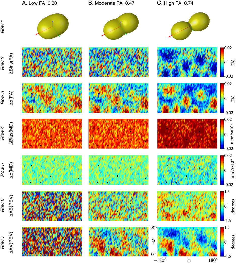
Simulated impact of DW scheme on tensor metrics for the PE6 scheme relative to the Jones30 scheme. Differential impact of DW schemes on the underlying tensors can be appreciated by comparing the orientation dependence of the precision and accuracy of each contrast for a tensor with low, moderate, and high FA.
In general, FA bias and precision were dependent on the orientation and anisotropy of the diffusion tensor. High anisotropy tensors exhibited greater changes in FA bias and precision (Fig. 10, rows 2 and 3 respectively) than lower anisotropy tensors. In particular, for tensors aligned with the DW directions, the magnitude of the FA bias tended to decrease and FA variability increase while for other orientations (aligned between DW directions), the magnitude of the FA bias increased and FA variability decreased.
The results for MD, on the other hand, did not show a strong relationship with the tensor alignment. The PE6 results were consistently more biased for all orientations. The difference in the magnitude of MD bias between PE6 and Jones30 protocol showed a slight increase for high FA tensors aligned with the DW directions (Fig. 10, row 4).
The precision and accuracy of the PEV orientation were dependent on the orientation and anisotropy of the tensor. In particular, tensors oriented collinear with the PE6 directions exhibited increased bias with PE6 relative to Jones30 (Fig. 10, row 6). The variability of PEV orientation decreased when the tensors were aligned with the sampling direction (Fig. 10, row 7). These effects were mitigated for moderate anisotropy tensors and were not visible with the low anisotropy tensors.
Simulation 3: impact of SNR on tensor estimation fidelity
SNR simulations indicate that estimation of FA is biased by the fiber orientation and directional resolution of the DW scheme. At very low SNR, there is up to a 0.12 [FA] bias as compared to estimates of FA for the high FA tensor; however, the magnitude of the bias decreases to less than 0.013 [FA] at 20 dB (Fig. 11, panel A). Both the percent and magnitude of the bias were smaller for more isotropic tensors. Variability of FA estimation was similar for the three tensors; the results for the high FA Tensor are shown. As expected, there was a consistent decrease in variability with increased SNR (Fig. 11, panel B). For all SNR levels, the variability was greatest when the tensor was in the lower FA bias orientation and imaged with 6 DW directions and least for the higher FA bias orientation when imaged with 6 DW directions. The variability of FA measurements with 30 DW directions consistently fell between these extremes with little differences between the orientations. Note that the difference in variability for orientations with the 6 DW directions is still 0.025 [FA] at 25 dB.
Fig. 11.

Simulated interactions of SNR, tensor orientation and DW scheme. Noise level and orientation demonstrate a differential impact on the precision and accuracy of diffusion tensor contrasts.
The simulated estimation fidelity of MD was insensitive to tensor orientation as can be appreciated in Fig. 11, panel C. The Jones30 observations were accurate above 15 dB for the high FA tensors and showed little bias for the moderate and low FA tensor at 10 dB. However, there is a substantial bias between MD estimated with PE6 and Jones30 at low SNR. This bias persists to moderate SNR and can be seen to be 2.2% for high FA tensors at 20 dB. The PE6 scheme demonstrated small, but consistently lower MD variability than the Jones30 with decreasing differences at high SNR. (Note that the circles are lower than the triangles in Fig. 11, panel D.)
Discussion
Selecting a diffusion weighting scheme
DTI results are systematically and statistically different when comparing studies using different, well-balanced DW schemes, a result that is in agreement with simulations. However, the magnitude of these differences is less than might be expected from other experimental parameters, such as changes in the number of DW images, number of averages, physiological noise, scanner hardware, or other factors that might influence the SNR. At 1 STE for example, using a DW scheme with 6 rather than 30 directions results in a differential orientation bias of approximately (1) 0.02 [FA] for FA, (2) 0.02 × 10⁻³ mm2/s for MD, and (3) 2° for PEV orientation. In order for these effects to be of clinical concern, they should be of the magnitude or greater than intra-session and inter-session reproducibility effects. In comparison for 1 STE with 30 directions, the intra-session test–retest variability of FA is ~ 0.1 [FA], MD is ~ 0.05 × 10⁻³ mm2/s, and PEV is ~ 5° (Farrell et al., 2006). In other words, compared to test–retest reproducibility and impact of SNR, the effects of the DW schemes are minor. We conclude that analyses from studies with different, but well-balanced DW scheme protocols are comparable.
When planning DTI studies, it is important to separate issues related to precision (reproducibility) and accuracy (bias) of each scheme. The optimized PE6, PE10, PE15 and Jones30 schemes tested in this study have comparable precision (e.g., Δσ in Fig. 8). This means that they have comparable powers to discriminate normal from abnormal. For group studies (ROI-based or voxel-based), these schemes should perform equally well. The bias becomes an issue if one needs to compare results between different DW schemes. If datasets are simply compared with values reported in the literature, the bias reported in this study should be a minor influence. However, if results from two different schemes are statistically compared within one study, great care should be exercised. The difference due to the PE6 and Jones30 DW schemes could be non-negligible when a group study is performed in brain regions with a specific fiber orientation, and the fiber is oriented in such a way that the diffusion weightings observed with the PE6 and Jones30 difference are maximally different. For example, suppose that 10 subjects are scanned once with each of two protocols, once with Jones30 and again with five repetitions of PE6. If one assumes good registration and anatomical correspondence, FA inter-session variability is ~ 0.1 [FA] (Farrell et al., 2006) with 1 STE (30 DWIs + 5 , approximately 3.5–4 min of scan time) and maximum orientation bias difference is ~ 0.03 [FA] (Fig. 7). A simple power analysis reveals that there is an 11% chance that a t-test would detect at least one significant difference due the bias (Altman, 1999). If 50 subjects are studied, the likelihood of detection increases to 54%. The amount of the bias decreases as the SNR increases (Fig. 11). Therefore, the difference could be harder to detect as the scan time increases. These conditions are met when the same subject is scanned on the same scanner. In reality, variability in group studies is dominated by variability among the subjects, scanner performance and image registration quality, which is not included in the above power analysis. Nonetheless, it is always advisable to use the same imaging parameters as much as possible for group studies. The choice of a diffusion weighting scheme should be recognized as one of the important parameters that should be considered.
In this study, cardiac gating was not applied. It is well known that cardiac pulsation can have a profound effect on DTI results (Golay et al., 2002; Jones and Pierpaoli, 2005), which could be a major contribution to the intra- and inter-session reproducibility noted in this study. Studies with cardiac gating should have better reproducibility and the relative significance of the PE6 −Jones30 difference, described above, may increase in such studies. Unfortunately, cardiac gating has not been widely accepted in clinical studies because it lengthens the scanning time and subject motion conditions and arrhythmia can occasionally cause gating instability.
When a protocol is being designed for a new study, a DW scheme with a larger number of gradient orientations should be considered because of the decreased directional sensitivity (little orientation dependence for precision and accuracy) even though the improvement could be minor, as has been demonstrated in this and previous (Jones, 2004) studies. However, schemes with fewer DW directions may have practical benefits that are not considered in this paper such as more efficient diffusion weighting. Repeated measurements (e.g., five repetition of PE6 as opposed to one Jones30 measurement) allow variability assessment among redundant datasets, which carry important information about image corruption and coregistration errors. Another example is that the observed signal can be increased by minimizing TE (Pierpaoli et al., 1996) or by applying a more efficient diffusion weighting scheme (Basser and Pierpaoli, 1996). For example, by changing from a PE6 scheme to a Tetra6 scheme, TE is reduced from 88 ms to 80 ms which corresponds to an 11% signal increase for white matter (assuming an approximate T2 of 80 ms). However, tradeoffs occur at the expense of increased condition number, hence noise propagation, and the benefit must be evaluated on a case by case basis (Batchelor et al., 2003; Skare et al., 2000). For example, the orientation variability for the PE6 results at 1 STE is lower than it is for the Tetra6 results at 3 STE, even though the SNR in the latter case is approximately greater (Fig. 8). Such a large increase in SNR cannot be achieved by TE shortening, indicating that the PE6 scheme will always yield better results than the Tetra6 scheme.
A simple multivariate log-linear least-square fitting method was used in this study. Recently, other fitting methods such as robust tensor estimation methods (Chang et al., 2005; Cox and Glen, 2006; Koay et al., 2006) have been introduced. Differences due to robust and simple tensor estimation methods are systematic (Koay et al., 2006), so caution must be used when comparing results from studies using different methods. It would be an interesting area of future research to evaluate if robust tensor estimation methods have consistent impacts on bias and variability depending on tensor orientation or DW scheme.
The close agreement of experimental and simulation results reinforces the general purpose utility of single tensor simulation models for investigating the performance of DTI protocols. The correspondence between the acquired and simulated data was especially strong for the variability measures and the patterns of orientation dependence. There is a possible discrepancy between Figs. 8 and 11. Namely, while the simulated data (Fig. 11) indicate that the bias between PE6 and Jones30 decreases as SNR goes up, the acquired data (1 STE versus 3 STE) indicate that the bias persists with a high SNR dataset (3 STE). We suspect that the bias at 3 STE (between the PE6 and Jones30 schemes) may not be mitigated by SNR and is due to non-tensor behavior (e.g., crossing fibers) seen in acquired MR data. Recently, Behrens et al. (2006) demonstrated that approximately one third of brain voxels satisfy the criteria for having multiple fiber populations. If there are a significant number of voxels with the non-tensor behavior, it is reasonable to expect that differences between PE6 and Jones30 results manifest as bias with respect to high SNR data because the gold standard was determined by using all data acquired with Jones30 scheme. This difference should be sensitive to b-value (the higher the b-value, the more pronounced the effect Frank, 2002). Nonetheless, the effect of non-tensor behavior is not considered in this article and is a fascinating future project.
Orientation analysis
In addition to conventional ROI-based analysis, we performed experiment (Fig. 7) and simulation-based (Fig. 9) orientation analysis. Even though many of the findings in this study simply confirmed results from previous simulation studies, we believe that it is an important effort to reconcile previous studies. FA, MD, and PEV showed consistent orientation patterns of bias and variability in both experiments and simulation data, as summarized in Table 1. FA precision and accuracy showed the greatest spatial dependence on the DW scheme, with a decrease in FA and increased variability roughly corresponding to DW directions. MD measurements were insensitive to DW scheme and thus to tensor orientation, while PEV measurements showed some dependence on DW scheme. The differences between the effect sizes and precise boundaries between the experimental and simulated data can be attributed to (1) spatially varying SNR, (2) differences between specified and realized DW directions, and (3) partial volume effects. As the sign, magnitude, and spatial patterns of the effects were highly consistent between simulation and acquired MR experiments, the data suggest that the single tensor model is useful for characterizing the behavior of differences between DW schemes.
Increasing the directional resolution of the DW scheme decreased the range of the orientation dependence for all contrasts (Fig. 8). This means that a DW scheme with more directions has a smooth precision and accuracy profile, which does not change profoundly as a function of fiber orientation. On average, low directional resolution showed increased FA and MD bias and variability. These effects are seen in Fig. 8 at both 1 and 3 STE ( SNR approximately 18 dB (7.9:1) and 20 dB (10:1)).
Single tensor simulations (Fig. 10) provide intuition on how aggregate profiles develop by considering mean behavior over ROIs. Orientation dependence is dominated by moderate and high FA tensors, as these tensors exhibit the greatest degree of orientation variability. FA bias decreased and variability increased for tensors aligned with the DW directions for PE6 relative to Jones30 (Fig. 10). Neither MD bias nor variability showed strong orientation dependence. The relationship between PEV, DW direction, and estimation reliability was complicated, however, in general AV tended to decrease and AB increase when the PEV was aligned with a DW direction.
The SNR tensor simulations demonstrate how these interactions generalize to other biological contexts or SNR levels (Fig. 11). At less than 15 dB (5.6:1), tensor estimation is exceptionally noisy, eigenvalues are notably biased, and there is substantial angular dependence introduced for the 6 DW direction scheme. At greater than 30 dB (31.6:1), neither minimal bias, orientation dependence, nor DW scheme dependence is apparent in either the FA or MD. Therefore, low SNR tends to exacerbate the orientation dependence of DTI contrast estimation and differences due to DW schemes.
Conceptualizing results
The results of this study are in agreement with Jones (2004) in that the error orientation profiles can be thought of “as a rubber sheet, and the sampling vectors as ‘fingers’” that serve to even out the surfaces. In other words, more independent sampling directions result in less orientation dependence in the precision and accuracy of derived quantities, when the total number of DW directions is held constant. Yet, these “fingers” are a bit more complex than weights on a surface serving to improve estimation.
The choice between sampling at independent directions versus repeated directions can be thought of as a tradeoff between shape (e.g., FA and MD) and orientation (e.g., PEV). The potential information about a tensor contained in a set of sampled DW directions is dependent on the tensor and noise. The results from this study (both simulation and in vivo measurements) show that estimation accuracy and precision of contrasts are not necessarily optimal for tensors aligned with the DW directions. This can be intuitively appreciated by considering a “diffusion peanut” for a prolate tensor (Jones and Basser, 2004). The physical diffusion process gives rise to a 3D diffusion profile, which is then sampled by DW imaging. The diffusion peanut is the conceptual representation of the diffusivity measured in each direction. In the case of a prolate tensor with high anisotropy, the derivatives of the spatial profiles of the diffusion peanut are relatively low at the poles and the equator. Sampling several locations (e.g., acquiring DW images with diffusion sensitization along these directions) in these regions would tell little about the orientation of the tensor, yet these would prove useful in determining anisotropy. Conversely, between the poles and equator, the profile of the diffusion peanut changes more rapidly, which well indicates orientation, but tells little about anisotropy. Furthermore, when noise is considered, different sampling directions may be determined with different accuracies due to varying signal attenuation and/or spatially varying SNR (e.g., due to parallel imaging techniques).
The results from this study agree with this analogy as we note that orientations of improved FA accuracy correspond to the orientations of decreased PEV accuracy. This effect can be thought of as a tradeoff between measuring the shape of the tensor and the orientation of the tensor. The high directional resolution scheme minimizes the variability for a tensor of unknown orientation, while a change to a low directional resolution scheme has varying impacts based on the orientation of the underlying tensor. If a DW scheme over samples slowly changing regions of the diffusion profile, the eigenvalues (hence, FA) will be relatively better determined. While if the rapidly changing regions of the diffusion profile are over sampled, the orientation (hence, PEV) will be relatively better determined. In light of this conceptual model, the experimental (Fig. 7) and simulation (Fig. 10) results are not surprising.
There clearly is inhomogeneity (orientation-dependent variation) in bias and variability. The inhomogeneity is not random and is related to sampling orientations. For FA, the maxima (or minima) correspond well to the sampling orientations, but for MD and PEV, the maxima or minima agree less well with the sampled orientations. In some cases, the perception of correspondence may be a function of the window-level of the figures. However, the phenomena are likely real, and may be explained by the contributions of all sampling directions and the secondary and tertiary eigenvectors.
Conclusion
This study characterizes how the number of directions in a DW scheme, impacts the precision and accuracy of in vivo fractional anisotropy (FA), mean diffusivity (MD) and principal eigenvector (PEV) findings and provides a principled theoretical framework to support and interpret the in vivo findings with simulation results. The observed differences in the DTI contrasts due to different DW schemes are shown to be small relative to intra-session variability. This result suggests that typical clinical studies, which use similar protocols but different DW schemes, are readily comparable within the experimental precision.
Acknowledgments
This research was supported by NIH grants NCRR P41RR15241 (Peter C.M. Zijl), RO1AG20012 (Mori), U24 RR021382-02 (Morphometry group of the Biomedical Informatics Research Network, BIRN, http://www.nbirn.net), and 1R01NS056307 (Prince). Dr. Craig K. Jones is supported by a grant from Philips Medical Systems to the Kennedy Krieger Research Institute. We greatly appreciate the feedback from our anonymous reviewers.
Appendix A. Precision and accuracy of the PEV orientation
Bias, variability and mean differences between PEV were assessed with metrics illustrated by the cartoons in Appendix Fig. A1. First, the mean PEV is computed in two steps: (1) all PEVs were reoriented (either rotated 180° or not) so that they were within 90° of the gold standard PEV, and (2) the mean PEV was computed by component-wise averaging, followed by normalization to unit length. The angular variability (AV) was computed as the mean angle between each observation and the mean PEV,
where denotes a vector dot product. Angular bias (AB) was defined as the mean angular differences between the mean PEV and the gold standard PEV,
Since the number of observations per voxel was limited in the region of interest studies, angular errors were assessed by the mean angular difference (MAD), which is the mean angular difference between each observation and the gold standard,
Note that the MAD metrics has contributions from both bias and variability. In analogy with the familiar bias, variance, mean square error (MSE) relationship:
The analogy holds well with the physical interpretations of the types of error. MAD and MSE are weighted averages of the distance of observations to the actual value. AV and variance are measures of spread of the observations about the observation mean, while AB and bias represent the distance from the observation mean to the actual value.
Fig. A1.

Illustration of angular error metrics. Angular variability (AV, panel A) is defined as the mean angle between observed vectors and the mean vector, while angular bias (AB, panel B) is defined as the angle between the mean vector and a gold standard (GS) reference vector. The mean angular difference (MAD, panel C) is defined as the mean angle between observed vectors and a gold standard. Ovals indicate the mean angle of the encompassed arcs.
Table A1.
Jones30 gradient table
| Index | Gx | Gy | Gz |
|---|---|---|---|
| 1 | 1.000 | 0.000 | 0.000 |
| 2 | 0.166 | 0.986 | 0.000 |
| 3 | −0.110 | 0.664 | 0.740 |
| 4 | 0.901 | −0.419 | −0.110 |
| 5 | −0.169 | −0.601 | 0.781 |
| 6 | −0.815 | −0.386 | 0.433 |
| 7 | 0.656 | 0.366 | 0.660 |
| 8 | 0.582 | 0.800 | 0.143 |
| 9 | 0.900 | 0.259 | 0.350 |
| 10 | 0.693 | −0.698 | 0.178 |
| 11 | 0.357 | −0.924 | −0.140 |
| 12 | 0.543 | −0.488 | −0.683 |
| 13 | −0.525 | −0.396 | 0.753 |
| 14 | −0.639 | 0.689 | 0.341 |
| 15 | −0.330 | −0.013 | −0.944 |
| 16 | −0.524 | −0.783 | 0.335 |
| 17 | 0.609 | −0.065 | −0.791 |
| 18 | 0.220 | −0.233 | −0.947 |
| 19 | −0.004 | −0.910 | −0.415 |
| 20 | −0.511 | 0.627 | −0.589 |
| 21 | 0.414 | 0.737 | 0.535 |
| 22 | −0.679 | 0.139 | −0.721 |
| 23 | 0.884 | −0.296 | 0.362 |
| 24 | 0.262 | 0.432 | 0.863 |
| 25 | 0.088 | 0.185 | −0.979 |
| 26 | 0.294 | −0.907 | 0.302 |
| 27 | 0.887 | −0.089 | −0.453 |
| 28 | 0.257 | −0.443 | 0.859 |
| 29 | 0.086 | 0.867 | −0.491 |
| 30 | 0.863 | 0.504 | −0.025 |
Table A2.
Partitions of the Jones30 gradient table
| Partitioning scheme | Indices of DW directions |
|---|---|
| Tetra6 | 8, 12, 13, 20, 21, 22 |
| PE6 | 5, 8, 11, 23, 24, 27 |
| PE10 | 1, 6, 8, 10, 12, 19, 22, 24, 25, 29 |
| PE15 | 2, 3, 4, 7, 11, 12, 13, 15, 20, 21, 23, 25, 27, 29, 30 |
Footnotes
Available online on ScienceDirect (www.sciencedirect.com).
References
- Alexander DC, Barker GJ, 2005. Optimal imaging parameters for fiber-orientation estimation in diffusion MRI. NeuroImage 27 (2), 357–367. [DOI] [PubMed] [Google Scholar]
- Altman DG, 1999. Practical Statistics for Medical Research. Chapman and Hall, CRC, New York. [Google Scholar]
- Basser PJ, Pierpaoli C, 1996. Microstructural and physiological features of tissues elucidated by quantitative-diffusion-tensor MRI. J. Magn. Reson., B 111 (3), 209–219. [DOI] [PubMed] [Google Scholar]
- Basser P, Mattiello J, LeBihan D, 1994. Estimation of the effective selfdiffusion tensor from the NMR spin echo. J. Magn. Reson., B 103 (3), 247–254. [DOI] [PubMed] [Google Scholar]
- Batchelor PG, Atkinson D, Hill DL, Calamante F, Connelly A, 2003. Anisotropic noise propagation in diffusion tensor MRI sampling schemes. Magn. Reson. Med 49 (6), 1143–1151. [DOI] [PubMed] [Google Scholar]
- Behrens TEJ, Berg HJ, Jbabdi S, Rushworth MFS, Woolrich MW, 2006. Probabilistic diffusion tractography with multiple fibre orientations: what can we gain? NeuroImage 34 (1), 144–155. [DOI] [PMC free article] [PubMed] [Google Scholar]
- Chang LC, Jones DK, Pierpaoli C, 2005. RESTORE: robust estimation of tensors by outlier rejection. Magn. Reson. Med 53 (5), 1088–1095. [DOI] [PubMed] [Google Scholar]
- Conturo TE, McKinstry RC, Akbudak E, Robinson BH, 1996. Encoding of anisotropic diffusion with tetrahedral gradients: a general mathematical diffusion formalism and experimental results. Magn. Reson. Med 35 (3), 399–412. [DOI] [PubMed] [Google Scholar]
- Cox R, Glen D, 2006. Efficient, robust, nonlinear, and guaranteed positive definite diffusion tensor estimation. Proceedings: International Society for Magnetic Resonance and Medicine, 14th Scientific Meeting, Seattle, WA, p. 349. [Google Scholar]
- Farrell JA, Landman BA, Jones CK, Smith SA, Prince JL, van Zijl PCM, Mori S, 2006. Effects of diffusion weighting scheme and SNR on DTI-derived fractional anisotropy at 1.5T. Proceedings: International Society for Magnetic Resonance in Medicine, 14th Scientific Meeting, Seattle, Washington, p. 1075. [Google Scholar]
- Frank LR, 2002. Characterization of anisotropy in high angular resolution diffusion-weighted MRI. Magn. Reson. Med 47 (6), 1083–1099. [DOI] [PubMed] [Google Scholar]
- Golay X, Jiang H, van Zijl PC, Mori S, 2002. High-resolution isotropic 3D diffusion tensor imaging of the human brain. Magn. Reson. Med 47 (5), 837–843. [DOI] [PubMed] [Google Scholar]
- Good PI, 2000. Permutation Tests: A Practical Guide to Resampling Methods for Testing Hypotheses. New York, Springer. [Google Scholar]
- Hasan KM, Parker DL, Alexander AL, 2001. Comparison of gradient encoding schemes for diffusion-tensor MRI. J. Magn. Reson. Imaging 13 (5), 769–780. [DOI] [PubMed] [Google Scholar]
- Hasan KM, Alexander AL, Narayana PA, 2004. Does fractional anisotropy have better noise immunity characteristics than relative anisotropy in diffusion tensor MRI? An analytical approach. Magn. Reson. Med 51 (2), 413–417. [DOI] [PubMed] [Google Scholar]
- Jenkinson M, Bannister P, Brady M, Smith S, 2002. Improved optimization for the robust and accurate linear registration and motion correction of brain images. NeuroImage 17 (2), 825–841. [DOI] [PubMed] [Google Scholar]
- Jones DK, 2003. Determining and visualizing uncertainty in estimates of fiber orientation from diffusion tensor MRI. Magn. Reson. Med 49 (1), 7–12. [DOI] [PubMed] [Google Scholar]
- Jones DK, 2004. The effect of gradient sampling schemes on measures derived from diffusion tensor MRI: a Monte Carlo study. Magn. Reson. Med 51 (4), 807–815. [DOI] [PubMed] [Google Scholar]
- Jones DK, Basser PJ, 2004. “Squashing peanuts and smashing pumpkins”: how noise distorts diffusion-weighted MR data. Magn. Reson. Med 52 (5), 979–993. [DOI] [PubMed] [Google Scholar]
- Jones D, Pierpaoli C, 2005. The contribution of cardiac pulsation to variability in tractography results. Proceedings: Internation Society on Magnetic Resonance in Medicine, 13th Annual Meeting, Miami, Florida, p. 225. [Google Scholar]
- Jones D, Williams S, Horsfield M, 1997. Full representation of whitematter fibre direction on one map via diffusion tensor analysis. Proceedings: International Society for Magnetic Resonance in Medicine, 5th Scientific Meeting, Vancouver, Canada, p. 1743. [Google Scholar]
- Jones DK, Horsfield MA, Simmons A, 1999. Optimal strategies for measuring diffusion in anisotropic systems by magnetic resonance imaging. Magn. Reson. Med 42 (3), 515–525. [PubMed] [Google Scholar]
- Koay CG, Chang LC, Carew JD, Pierpaoli C, Basser PJ, 2006. A unifying theoretical and algorithmic framework for least squares methods of estimation in diffusion tensor imaging. J. Magn. Reson 182 (1), 115–125. [DOI] [PubMed] [Google Scholar]
- Landman BA, Farrell JAD, Mori S, van Zijl PCM, Prince JL, 2006. On the coregistration of diffusion weighted images. Proceedings: International Society for Magnetic Resonance in Medicine, 14th Scientific Meeting, Seattle, Washington, p. 2987. [Google Scholar]
- Muthupallai R, Holder C, Song A, Dixon W, 1999. Navigator aided, multishot EPI diffusion images of brain with complete orientation and anisotropy information. Proceedings: International Society for Magnetic Resonance in Medicine, 7th Scientific Meeting, Philadelphia, Pennsylvania, p. 1825. [Google Scholar]
- Ni H, Kavcic V, Zhu T, Ekholm S, Zhong J, 2006. Effects of number of diffusion gradient directions on derived diffusion tensor imaging indices in human brain. AJNR Am. J. Neuroradiol 27 (8), 1776–1781. [PMC free article] [PubMed] [Google Scholar]
- Papadakis NG, Xing D, Houston GC, Smith JM, Smith MI, James MF, Parsons AA, Huang CLH, Hall LD, Carpenter TA, 1999. A study of rotationally invariant and symmetric indices of diffusion anisotropy. Magn. Reson. Imaging 17 (6), 881–892. [DOI] [PubMed] [Google Scholar]
- Pierpaoli C, 1997. Oh no! One more method for color mapping of fiber tract direction using diffusion MR imaging data. Proceedings: International Society for Magnetic Resonance in Medicine, 5th Scientific Meeting, Vancouver, Canada, p. 1741. [Google Scholar]
- Pierpaoli C, Jezzard P, Basser PJ, Barnett A, Di Chiro G, 1996. Diffusion tensor MR imaging of the human brain. Radiology 201 (3), 637–648. [DOI] [PubMed] [Google Scholar]
- Skare S, Hedehus M, Moseley ME, Li TQ, 2000. Condition number as a measure of noise performance of diffusion tensor data acquisition schemes with MRI. J. Magn. Reson 147 (2), 340–352. [DOI] [PubMed] [Google Scholar]
- Stejskal EO, Tanner JE, 1965. Spin diffusion measurements: spin echoes in the presence of a time-dependent field gradient. J. Phys. Chem 42, 288–292. [Google Scholar]