



Abstract
Objectives:
This study aimed to determine the speech-to-background ratios (SBRs) at which normal-hearing (NH) and hearing-impaired (HI) listeners can recognize both speech and environmental sounds when the two types of signals are mixed. Also examined were the effect of individual sounds on speech recognition and environmental sound recognition (ESR), and the impact of divided vs. selective attention on these tasks.
Design:
In Experiment 1 (divided attention), 11 NH and 10 HI listeners heard sentences mixed with environmental sounds at various SBRs and performed speech recognition and ESR tasks concurrently in each trial. In Experiment 2 (selective attention), 20 NH listeners performed these tasks in separate trials. Psychometric functions were generated for each task, listener group, and environmental sound. The range over which speech recognition and ESR were both high was determined, as was the optimal SBR for balancing speech recognition with ESR, defined as the point of intersection between each pair of normalized psychometric functions.
Results:
The NH listeners achieved greater than 95% accuracy on concurrent speech recognition and ESR over an SBR range of approximately 20 dB or greater. The optimal SBR for maximizing both speech recognition and ESR for NH listeners was approximately +12 dB. For the HI listeners, the range over which 95% performance was observed on both tasks was far smaller (span of 1 dB), with an optimal value of +5 dB. Acoustic analyses indicated that the speech and environmental sound stimuli were similarly audible, regardless of the hearing status of the listener, but that the speech fluctuated more than the environmental sounds. Divided versus selective attention conditions produced differences in performance that were statistically significant yet only modest in magnitude. In all conditions and for both listener groups, recognition was higher for environmental sounds than for speech when presented at equal intensities (i.e., 0 dB SBR), indicating that the environmental sounds were more effective maskers of speech than the converse. Each of the 25 environmental sounds used in this study (with one exception) had a span of SBRs over which speech recognition and ESR were both higher than 95%. These ranges tended to overlap substantially.
Conclusions:
A range of SBRs exists over which speech and environmental sounds can be simultaneously recognized with high accuracy by NH and HI listeners, but this range is larger for NH listeners. The single optimal SBR for jointly maximizing speech recognition and ESR also differs between NH and HI listeners. The greater masking effectiveness of the environmental sounds relative to the speech may be related to the lower degree of fluctuation present in the environmental sounds as well as possibly task differences between speech recognition and environmental sound recognition (open vs. closed set). The observed differences between the NH and HI results may possibly be related to the HI listeners’ smaller fluctuating masker benefit. As noise-reduction systems become increasingly effective, the current results could potentially guide the design of future systems that provide listeners with highly intelligible speech without depriving them of access to important environmental sounds.
INTRODUCTION
Listening often occurs in the presence of multiple sound sources. Under these conditions, the acoustic wave that arrives at each ear contains a mixture of sounds. When sounds originate from different directions relative to the listener’s head, binaural cues can aid in perceptually segregating a signal of interest from the other sound(s) in the auditory scene (Bregman 1990). However, in what may be described as a “worst-case scenario” where sounds arrive from the same direction, the listener must rely primarily on monaural cues to segregate sounds. For humans, the speech of a target talker is often the signal of interest. Because other sounds can reduce speech recognition via masking, they are traditionally considered to be the “noise,” “interference,” “masker,” or “background.”
An extensive body of research has examined speech recognition in the presence of a wide variety of masker types, including sine waves, square waves, and repetitive pulses (Stevens et al. 1946); warbling tones, music, band pass filtered noise, amplitude-modulated noise, frequency-modulated noise, peak-clipped noise, gated noise, and one or more competing talkers (Miller 1947); white noise (Hawkins & Stevens 1950; Fletcher 1953); complex tones (Licklider & Guttman 1957); speech-shaped noise (Busch & Eldredge 1967); speech-modulated speech-shaped noise (Brungart 2001); spectro-temporally modulated noise (Howard-Jones & Rosen 1993; Fogerty et al. 2018); environmental sounds such as naval ship noises (Klumpp & Webster 1963) and aircraft noise (Kryter & Williams 1966); and complex soundscapes such as cafeteria noise (Cooper & Cutts 1971) and traffic noise (Aniansson 1978). Speech recognition for listeners with normal hearing (NH) is largely unaffected by broadband noise so long as the signal to noise ratio is at least 6 dB, and performance can remain above chance even when the signal to noise ratio is as low as −18 dB (Licklider & Miller 1951). The effect of noise on speech recognition for hearing-impaired (HI) listeners tends to be greater, and the magnitude of this effect largely depends on the degree, type, and configuration of hearing loss (Ross et al. 1965).
In realistic listening situations, however, the speech of a single target talker may not always be the only signal of interest in an acoustic mixture. When environmental sounds are present, they provide information about objects and events around the listener. Environmental sounds not only contribute to listeners’ sense of awareness and well-being (Ramsdell 1978; Jenkins 1985; Reed & Delhorne 2005) but also warn of potential dangers in the environment (e.g., approaching vehicles, sirens, falling objects). When a relevant environmental sound overlaps with target speech, each is both signal and masker because each is of interest to the listener, and each has the potential to interfere with the perception of the other. Because of this, the term “speech-to-background ratio” (SBR) will be used in place of “signal-to-noise ratio” in the present study to express the amplitude relationship between speech and concurrent environmental sound.
In addition to situations where speech and environmental sounds are both of interest to the listener, there may be instances where concurrent sounds are present but only one is a signal of interest. Such cases call for selective attention, which refers to cognitive processes that enable an individual to attend to specific stimuli for further processing while suppressing irrelevant or interfering information from the environment. For example, sound sources that the listener considers unimportant, uninteresting, or disturbing, such as the revving of a neighbor’s chainsaw during a conversation with a friend, are often not the target of the listener’s attention. At other times, however, an environmental sound could be the primary signal of interest while speech plays the role of interference (e.g., an alarm sounding or car approaching while someone is talking). A number of studies have investigated how humans recognize environmental sounds in quiet (Lawrence & Banks 1973; Lass et al. 1982; Gygi and Shafiro 2010a) and in the presence of competing sounds (Ballas & Mullins 1991; Niessen et al. 2008; Leech et al. 2009; Gygi & Shafiro 2011).
Although many studies have examined speech recognition in the presence of competing noise, few if any have considered environmental sound recognition (ESR) in the presence of competing speech. The present study is concerned with both of these aspects of auditory perception and the conditions under which both are possible. It is known that speech recognition improves toward ceiling performance as SBR increases. Inversely, it is presumed that ESR decreases toward the performance floor with increasing SBR. There should thus exist a trade-off between speech recognition and ESR as SBR varies. In the context of this trade-off, the present study aims to answer the following primary questions:
Is it possible to jointly obtain high speech recognition and high ESR at some SBR?
If yes, what is the optimal SBR for jointly maximizing speech recognition and ESR for NH listeners, and is there a range of SBRs over which speech recognition and ESR are both high?
Are joint speech recognition and ESR also possible for HI bilateral hearing aid users? And, if yes, do the optimal SBR values and ranges differ for NH versus HI listeners?
Does the optimal SBR value depend on the type of background sound?
The answers to these questions will further our understanding of auditory perception in normal and impaired systems. Moreover, since ESR is an important priority for adults with hearing loss (Bell 2005), the knowledge gained in this study could inform the design of future hearing devices, with the eventual aim of presenting signals at an “optimal” SBR, one that appropriately balances high speech recognition while also allowing for high ESR.
A secondary question involves the costs associated with performing two tasks simultaneously (divided attention). There are often limitations on listeners’ abilities to process all available auditory information in parallel, and divided attention concerns the allocation of cognitive resources between different signals by splitting or rapidly shifting attentional focus (Parasuraman 1998). Numerous studies have examined the human performance costs associated with divided attention when both tasks are speech recognition (e.g., Humes et al. 2006; Gallun et al. 2007; Apoux et al. 2018; Fumero et al. 2022). The present study provides an initial look into whether divided attention results in similar performance costs when one of the tasks is ESR, which likely involves a different set of auditory processing mechanisms (Lewis et al. 2004).
In Experiment 1, subjects performed speech recognition and ESR concurrently (divided attention). In Experiment 2, they performed each task separately (selective attention). Both experiments were concerned with listeners’ auditory perception in the absence of binaural cues, in accord with the “worst-case scenario” for sound source segregation. To address the questions listed above, psychometric functions were generated for each task in each condition or for each listener group.
Experiment 1
In Experiment 1, listeners were instructed to attend to both the speech and the environmental sound on each trial. This represents a dual-task paradigm that is likely more challenging than the many everyday listening situations in which listeners selectively attend to only one sound source at a time. It therefore also likely represents a lower bound for performance for these particular tasks.
MATERIALS AND METHODS
Subjects
Two groups of listeners participated. The first group was composed of 11 adults with NH, defined as pure-tone audiometric thresholds at 20 dB hearing level (HL) or lower at octave frequencies from 250 to 8000 Hz (ANSI 2004, 2010). The 2 exceptions involved 1 listener with a threshold of 25 dB HL at 1000 Hz in 1 ear and another listener with a threshold of 30 dB HL at 8000 Hz in 1 ear. The NH subjects were recruited from undergraduate courses and received course credit for participating. Ages ranged from 18 to 20 years (mean = 20), and all were female. Young listeners with NH were selected for the current task to represent ideal human performance.
The second group consisted of 10 HI listeners who were recruited from The Ohio State University Speech-Language-Hearing Clinic and selected to represent a diverse sample of adults who wear hearing aids. Accordingly, they were all binaural hearing aid users with varying degrees of bilateral sensorineural hearing loss. Hearing status was confirmed on the day of test using pure-tone audiometry (ANSI 2004, 2010) on a GSI Pello Audiometer (Eden Prairie, MN) with RadioEar DD45 earphones (Middelfart, Denmark) in a double-walled sound-attenuating booth. Pure-tone average thresholds, based on audiometric thresholds at 500, 1000, 2000, and 4000 Hz and averaged across ears, ranged from 19 to 63 dB HL with a mean of 34. HI subjects were numbered in order of increasing pure-tone average threshold (i.e., higher subject numbers correspond to greater mid-frequency hearing loss). Each audiogram displayed in Fig. 1 is labeled with an HI listener’s subject number, age, and sex. Ages ranged from 27 to 67 years (mean = 51), with 6 females and 4 males. HI subjects received a monetary incentive for participating.
Fig. 1.
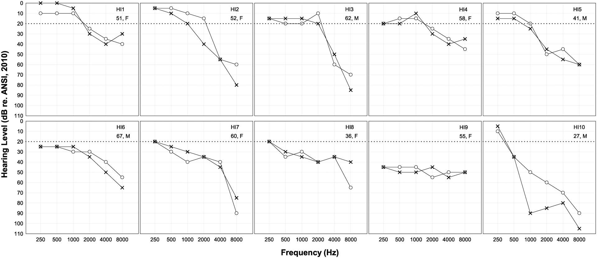
Pure-tone air-conduction audiometric thresholds for the hearing-impaired listeners. Listeners are numbered in order of increasing degree of hearing loss. Right ears are represented by circles and left ears are represented by X’s. The limit of normal hearing (20 dB HL) is represented by a dotted horizontal line in each panel. Subject numbers, ages in years, and sexes are also provided.
All participants were native speakers of American English, and none had any previous experience with the sentences used in this study. All participants gave their informed written consent to participate in this research, which was approved by the Institutional Review Board (IRB) at The Ohio State University.
Stimuli
Each stimulus consisted of a sentence mixed with an environmental sound. Sentences were drawn from the standard recording of the Hearing in Noise Test (HINT; Nilsson et al. 1994) and were all produced by an adult male speaker of General American English.
Environmental sounds were sourced from the Database of Environmental Sounds for Research Activities (Gygi & Shafiro 2010b), the Sound Effects Recognition Test (Finitzo-Hieber et al. 1980), a commercial stock media website (Pond5.com), and field recordings. The 25 sounds selected for this study were judged by the researchers to be familiar to the general population and sufficiently distinct from each other to minimize confusion between sounds. It is important to note that the duration of each environmental sound was greater than or equal to the longest sentence stimulus used in the study. This ensured that sounds were capable of masking entire sentences via simultaneous masking. Thus, short-duration sounds such as isolated transients (e.g., a single knock at the door) were not used. However, sounds were allowed to vary with regard to degree of modulation, and some sounds were included (such as “drum”) that could be considered a series of transients. No other selection criteria were in place beyond these involving recognizability and relatively steady state nature. Figure 2 shows the graphical user interface used in this study, along with the name and graphic used for each sound.
Fig. 2.
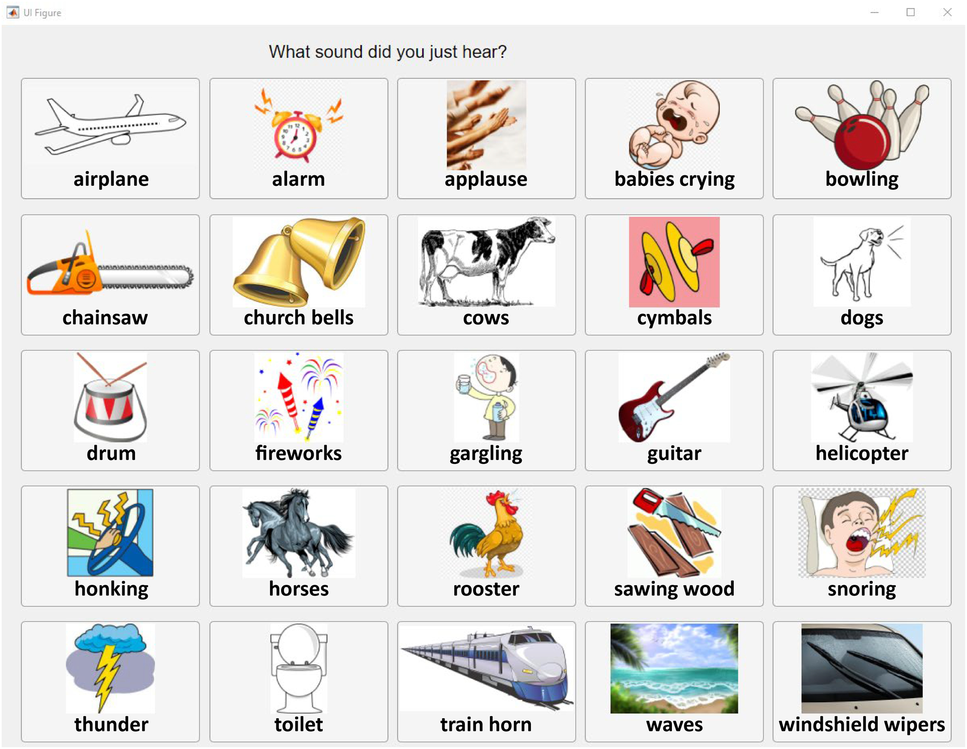
The graphical user interface used to record listener responses for environmental sounds. The 25 environmental sounds were arranged in a 5 × 5 grid in alphabetical order. Pictures were provided to assist in locating the appropriate response button.
The environmental sound mixed with the sentence was chosen randomly for each stimulus trial and subject. Stimuli were mixed at the following 10 SBRs: −36, −30, −8, −4, 4, 20, 32, 40, 64, and 70 dB. These SBRs were selected based on pilot testing to produce the entire range of floor to ceiling scores for both speech recognition and ESR, with at least two points on the steep portion and two points on the lower asymptote of each psychometric function.
Before to mixing, silence was trimmed from the beginning and end of each sentence and environmental sound so that their onsets aligned, thus eliminating any precursor or preceding fringe containing only speech or only background. Next, the length of the environmental sound was trimmed to match the length of the sentence, thus aligning their offsets and eliminating glimpses containing only the background sound at the end of each stimulus. Subjective listening by the authors revealed no audible onset/offset clicks following the trimming of ongoing sounds. The environmental sound was then scaled to achieve the desired SBR (based on root mean square [RMS] values) and mixed with the sentence. Finally, each mixture was scaled to the same RMS value. No time or frequency weighting was used in the RMS calculations. Because the overall level was held constant, the speech level was reduced for lower SBRs, and the environmental-sound level was reduced for higher SBRs. The sampling rate and bit depth of all stimuli were 44.1 kHz and 16 bits, respectively.
Procedure
Each subject heard a total of 250 stimuli in a single session, blocked by the 10 SBR conditions, with 25 stimuli per condition. The SBRs were presented in a random order for each subject, whereas the sentences were presented in the same fixed order for each subject. Again, the background sound was chosen randomly, with replacement, for each subject on each experimental trial. Thus, there were always 25 possible background sounds for each trial, and a given sound could be used repeatedly or not at all in a condition. But on average across listeners, each environmental sound was presented once per listener per SBR.
Listeners were tested individually in a double-walled audiometric booth, seated in front of a computer monitor and mouse. The experimenter was also seated in the booth, approximately six feet from the listener. Listeners were instructed to perform two tasks on each trial containing a sentence mixed with an environmental sound: First, repeat the sentence out loud; then, click on the labeled picture corresponding to the background sound in the stimulus (Fig. 2), guessing on either task if unsure. Listeners were instructed to perform the tasks in this order to ensure they fully completed their spoken response before the onset of the subsequent stimulus presentation, which occurred 300 ms after clicking the button representing their environmental-sound response. The experiment was thus self-paced. The experimenter recorded the number of words correctly reported for each sentence while listeners’ responses to the ESR task were recorded in a custom MATLAB application (version 2019a; MATLAB 2019). Both the listener and experimenter were blind to the conditions under test. No feedback was provided to listeners during formal testing.
Stimuli were played back on a Windows PC, converted to analog form using an RME Fireface UCX audio interface (Haimhausen, Germany), amplified using a Mackie 1202-VLZ mixer (Woodinville, WA), and presented diotically over Sennheiser HD 280 Pro headphones (Wedemark, Germany). Hearing-impaired listeners were tested without their hearing aids. The level of each stimulus was set to 65 dBA (based on the equivalent continuous sound pressure level of a representative looped stimulus) in each ear for the NH subjects and verified using a sound-level meter and flat-plate coupler (Larson Davis models 824 and AEC 101, Depew, NH). For the HI listeners, additional individualized frequency-specific gains, as prescribed by the NAL-RP formula (Byrne et al. 1990), were applied to this 65 dBA presentation level, to compensate for their hearing loss. These gains were implemented using a RANE DEQ 60L digital equalizer (Mukilteo, WA), as described in Healy et al. (2015). The sound pressure level following NAL-RP amplification did not exceed 96 dBA for any participant.
Before to the start of formal testing, each participant completed a three-stage familiarization. The first stage involved learning to recognize the 25 background sounds in the absence of any competing speech. Participants heard each of the 25 background sounds, presented in a random order, and were instructed to click on the labeled picture representing the sound. Feedback was provided for any incorrect responses during this first stage of familiarization. The process was repeated (up to three times) until the listener could accurately identify each sound without correction or prompting from the experimenter. Across listeners, an average of two repetitions was required for perfect performance. One potential subject who could not perform this task (an older adult male with hearing loss) was dismissed from the experiment. In the second stage of familiarization, listeners heard seven HINT sentences in quiet and repeated each one out loud. In the third familiarization stage, listeners heard seven new HINT sentences mixed with a random background sound at each of the following SBRs, in this order: 12, −8, and 40 dB. Listeners were instructed to repeat back as much of each sentence as possible and then click on the picture representing the background sound, taking their best guess if unsure. The 28 HINT sentences used for familiarization were distinct from the 250 used for testing. Following the three familiarization stages, formal testing began, as described above. In total, each experimental session lasted approximately one hour.
Data Analysis
Psychometric functions based on the cumulative normal function were fit for each task type (speech recognition and ESR) and listener group using the quickpsy package (Linares & López-Moliner 2016) in R 4.1.3 (R Core Team 2022). Thus, the equation for each psychometric function for speech recognition was of the form:
| (1) |
And each psychometric function for ESR was of the form:
| (2) |
Where is the probability of correctly responding at an SBR of x dB, is the guess rate, is the lapse rate, and is a sigmoidal-shape function with asymptotes at 0 and 1, which in this case is the cumulative normal function. The mean of the cumulative normal distribution corresponds to the inflection point (50% threshold assuming no lapses or correct guesses) for the psychometric function, and the standard deviation of the distribution is reflected in the steepness of the psychometric function.
For each function, the explanatory variable was SBR, and the response variable was either words or environmental sounds correctly reported. The lapse rate (i.e., the probability of an incorrect response, independent of stimulus intensity) was calculated as a free parameter. The guess rate was set to 0% for the speech-recognition functions and to 4% (i.e., 1/25) for the ESR functions, representing chance performances. The range of each function was then normalized (i.e., rescaled) such that the lower asymptote (guess rate) was mapped to 0% correct, and the upper asymptote was mapped to 100% correct (0% lapse rate). This normalization was necessary because of the asymptotic nature of psychometric functions. In order to locate an SBR that balances speech recognition with ESR, a single point of intersection occurring as close as possible to the asymptotic ceiling for each function was sought. However, if the two functions have different ceiling levels, they will fail to intersect at each other’s asymptotes, even if they overlap in SBR. In other words, without normalization, the point of intersection skews toward the steep portion of the function with the lower lapse rate (higher upper asymptote). The magnitudes of the lapse rates are described below, reflecting the fact that normalization refined but did not largely modify the psychometric functions.
RESULTS
Figure 3 displays normalized psychometric functions for speech recognition and ESR based on the performance of the 11 NH listeners.
Fig. 3.
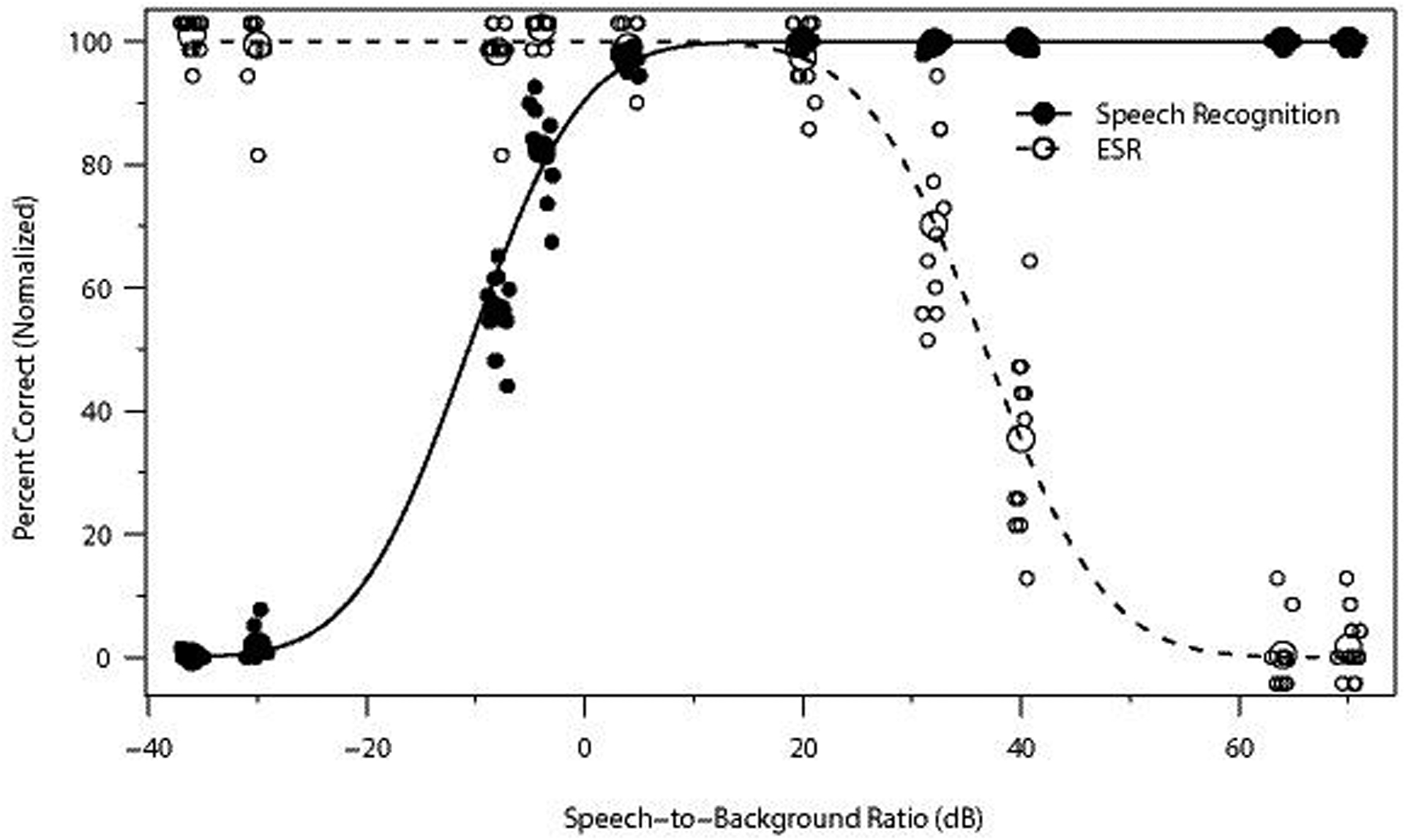
Normalized psychometric functions for speech recognition and ESR in conditions of divided attention based on the pooled performance of 11 normal-hearing listeners. Filled circles denote normalized percent words correct speech recognition, and open circles correspond to normalized percent correct ESR. Larger circles represent normalized group-mean performance, and smaller circles, which have been jittered for clarity, represent normalized mean performance values for individual participants at each speech-to-background ratio. The solid black line is the fitted psychometric function for speech recognition, and the dashed line is the fitted function for ESR. ESR indicates environmental sound recognition.
The estimated lapse rate for NH speech recognition was 0.05% (95% CI [0.0095%, 0.11%]). The threshold for 50% normalized speech recognition was −10.7 dB SBR (95% CI [−11.0, −10.2]), and the threshold for 95% normalized speech recognition was 2.8 dB SBR (95% CI [2.3, 3.3]).
The estimated lapse rate for NH ESR was 2.7% (95% CI [1.98%, 3.45%]). To account for chance performance, 4% (i.e., 1/25) was shifted to 0. The NH listeners’ normalized threshold for 50% correct ESR was 36.7 dB SBR (95% CI [35.8, 37.7]). The normalized threshold for 95% correct ESR was 22.4 dB SBR (95% CI [19.4, 24.7]).
Thus, the range (horizontal distance in Fig. 3) between NH listeners’ normalized 50% correct threshold for speech recognition and that for ESR was 47.4 dB (−10.7 to 36.7 dB SBR), whereas the range between their 95% correct thresholds spanned 19.6 dB (2.8 to 22.4 dB SBR). Since performance for both tasks was high (95% correct or greater) for all SBRs within these latter limits, any SBR bounded by 2.8 and 22.4 dB could be regarded as essentially optimal for maximizing both speech recognition and ESR. However, a single optimal value may be calculated as the point of intersection between the two normalized psychometric functions. This value is 12.2 dB SBR, where predicted normalized performance for both speech recognition and ESR converge at 99.7% correct (unnormalized speech recognition = 99.7 % correct; unnormalized ESR = 97.0% correct).
Figure 4 displays normalized psychometric functions for the group of 10 HI listeners who participated in this study. As in Fig. 3, normalized mean percent-correct values are plotted as a function of SBR for both speech recognition and ESR. For the HI listeners, the estimated lapse rate for speech recognition was 0.5% (95% CI [0.38%, 0.71%]). The HI listeners’ normalized 50% threshold for speech recognition was −6.7 dB SBR (95% CI [−7.0, −6.3]), and their normalized 95% threshold was 4.7 dB SBR (95% CI [3.9, 5.4]).
Fig. 4.
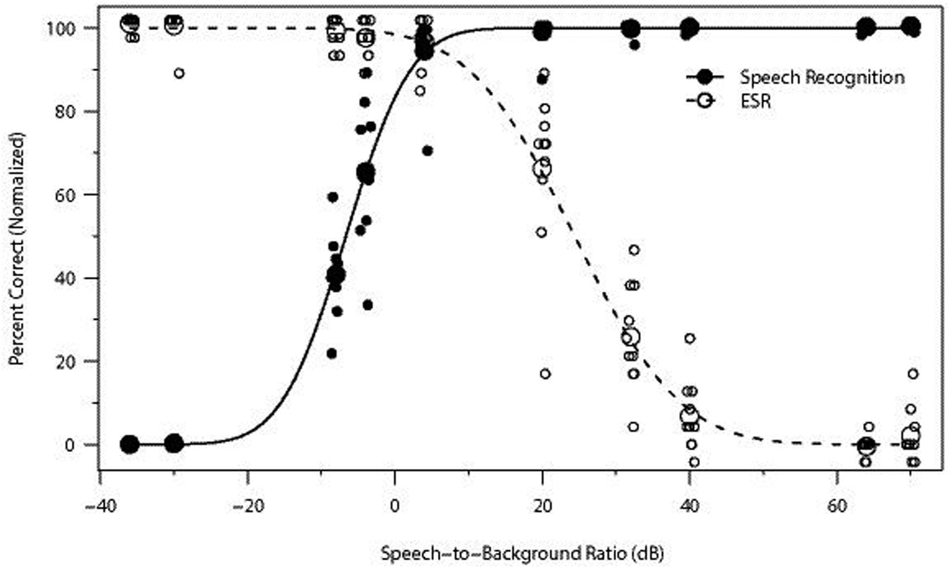
As Fig. 3, but for the 10 hearing-impaired listeners.
For ESR, the estimated HI lapse rate was 1.8% (95% CI [0.9%, 2.8%]). Normalized HI 50% and 95% thresholds for ESR were 24.2 (95% CI [23.2, 25.5]) and 5.8 dB SBR (95% CI [3.5, 8.6]), respectively. The estimated range between normalized 50% thresholds for speech recognition (−6.7 dB SBR) and ESR (24.2 dB SBR) for these HI listeners was 30.9 dB. There was also a narrow 1.1-dB range between which the HI listeners’ normalized thresholds for speech recognition and ESR were both above 95% correct. This range extended between 4.7 and 5.8 dB SBR. For these HI listeners, the optimal SBR for balancing the trade-off between speech recognition and ESR, when both are considered equally important, was calculated to be 5.1 dB, which is the point where the two psychometric functions in Fig. 4 intersect, at 95.6% normalized percent correct. It is further noted that other SBRs may be preferred when speech recognition is prioritized. For example, at 10 dB SBR, normalized speech recognition is above 99% correct while normalized ESR remains relatively high at 90% correct.
Compared to the NH listeners, the HI listeners displayed a narrower range over which concurrent performance was high. The HI listeners’ group threshold for 50% speech recognition was 4.0 dB higher (poorer) than the 50% correct threshold for the NH group. The difference between the HI and NH groups was even more pronounced for ESR. For this task, the HI group threshold for 50% correct was 12.5 dB lower (poorer) than the NH group threshold. Thus, it appears that the smaller range over which the HI listeners were able to recognize both speech and environmental sounds was more driven by an inward shift of the psychometric function for ESR than by an inward shift of the speech-recognition function. This suggests that ESR is considerably more affected than speech recognition for HI relative to NH listeners in the current concurrent-sound conditions.
Hearing-impaired and NH listeners also differed in terms of their optimal SBR for maximizing both speech recognition and ESR. This value was 5.1 dB for the HI listeners and 12.2 dB for the NH listeners. Although these particular values differ for NH vs. HI listeners, the optimal value for either listener group still allows concurrent normalized speech recognition and ESR to exceed 96% correct for both groups.
To compare the differences between the NH and HI subject groups, two mixed-effects logistic models were constructed in R 4.1.3 (R Core Team 2022) using the lme4 (Bates et al. 2014) and lmerTest (Kuznetsova et al. 2017) packages. In the first model, the outcome variable was binary data for words correct (n = 27,838 observations), and the fixed effects were SBR, listener type (NH or HI), and their interaction. SBR was expressed in dB units that were otherwise untransformed, and listener type was deviation coded, with NH coded as 0.5 and HI coded as −0.5. The model included random intercepts for listener and sentence. Models for speech recognition that included random intercepts for environmental sounds or random slopes failed to converge.
In the second model, the outcome variable was binary data for environmental sounds correct (n = 5,250 observations). This model also had fixed effects for SBR (in dB), listener type, and their interaction. As in the first model, listener type was deviation coded. The model for ESR included random intercepts for sentence, listener, and environmental sound. Models that included random slopes failed to converge.
Unsurprisingly, the effect of SBR was large and significant in both models. Increases in SBR reliably predicted higher speech recognition (β = 0.21, SE = 0.004, z = 49.6, p < 0.001) and lower ESR performance (β = −0.11, SE = 0.003, z = −32.7, p < 0.001).1 The main effect of listener type was significant for both speech recognition (β = 0.67, SE = 0.24, z = 2.80, p = 0.005) and ESR (β = 1.02, SE = 0.24, z = 4.22, p < 0.001) with NH listeners scoring higher overall on both tasks. The interaction between SBR and listener type was significant in the ESR model, but not in the speech-recognition model. For ESR, HI listeners benefitted from more favorable (lower) SBRs to a greater extent than did NH listeners (β = 0.012, SE = 0.005, z = −2.11, p = 0.035). Changing the SBR had an equally strong effect on both NH and HI speech recognition, (β = −0.01, SE = 0.007, z = −1.39, p = 0.16), but again, overall speech recognition was still higher for the NH subjects.
Audibility Analysis
The HI group’s performance was more dissimilar to the NH group’s performance on the ESR task than it was on the speech recognition task. One possible explanation for this finding is that the environmental sounds were simply less audible than the speech for the HI listeners. To examine this possibility, an audibility analysis was performed using the Speech Intelligibility Index (SII; ANSI S3.5–1997 1997). The SII estimates the amount of a given speech signal that is audible to a listener. It should be noted that the SII alone does not provide an estimate of percent-correct human recognition performance, especially for environmental sounds. The purpose of this audibility analysis, however, is not to predict recognition performance or model the results of Experiment 1; it is to compare the present speech and environmental sound signals in terms of their audibility in order to rule out the role of audibility in the results of Experiment 1. The SII was calculated for the separate speech and environmental sound components of each mixture heard by each listener, taking into account each HI listener’s audiometric thresholds and frequency-specific NAL-RP gains. For the NH listeners, 0 dB HL thresholds were assumed at all frequencies. Details of this analysis, including citations for Gygi et al. (2004) as well as Müsch and Zurek (2005), may be found in the Supplemental Appendix.
Sigmoid functions fit to the SII data representing the NH conditions were essentially symmetrical, with inflection points (equivalent to 50% thresholds) located at levels where the SBRs would be −36.2 dB for speech and +36.2 dB for environmental sounds. Sigmoid functions for the HI conditions were also nearly symmetrical, with inflection points occurring where the SBRs would be −21.0 dB for speech and +20.0 dB for environmental sounds. A comparison of these functions reveals a 15.2-dB inward shift (NH versus HI) of the SII function for speech and a 16.2-dB inward shift of the SII function for environmental sounds. Thus, the substantially larger inward shift (NH versus HI) for ESR performance (of 12.5 dB) relative to that shift for speech recognition (of 4.0 dB) in Fig. 3 versus Fig. 4 does not appear to be accounted for by differences in audibility for environmental sounds compared to speech. However, it should be noted that this audibility analysis is based on the long-term average spectra of the signals and did not take temporal fluctuations or signal dynamic range into account.
Percentile Analysis of Time-Dependent Level Changes
Another possible explanation for the differential effect of hearing loss on ESR vs. speech recognition involves the temporal characteristics of the stimuli and the reduced fluctuating-masker benefit frequently observed in HI listeners relative to NH listeners. Individuals with sensorineural hearing loss often struggle to understand speech in the presence of fluctuating background noise or a competing talker. Unlike NH listeners, HI listeners typically experience little speech recognition improvement in fluctuating noise environments compared to stationary maskers when both types of noise are at the same long-term sound pressure level (e.g., Bacon et al. 1998; Bernstein & Grant 2009; Ozmeral et al. 2016). Therefore, if the speech stimuli are more fluctuating than the environmental sounds, the HI listeners may have been less able to take advantage of the dips in the speech signal, resulting in poorer ESR performance.
To investigate this possibility, a short-time level percentile analysis was performed, as described in IEC 60118–15 (2012). Each set of stimuli (speech or environmental sounds) was concatenated into a single file without pauses and filtered into 1/3-octave bands. The output of each filter was then cut into 125-ms windows with 50% overlap, and the level of each window was calculated. The distributions of these short-term levels are the basis of the percentile analysis. Narrower distributions correspond to greater signal stationarity, and broader distributions correspond to greater signal fluctuation. Figure 5 shows long-term average spectra (black lines) and level frequency diagrams (based on percentile analysis) of the speech stimuli (left panel) and environmental sounds (right panel). The 30th percentile of each short-time level distribution, represented by the lower borders of the blue boxes, corresponds to the less-intense parts of the signal. The 65th percentile (border between the blue and red boxes) is similar to the average level, and the 99th percentile (upper border of the red boxes) describes the peaks of the signal. The difference between the 99th and 30th percentile describes the dynamic range of the signal.
Fig. 5.
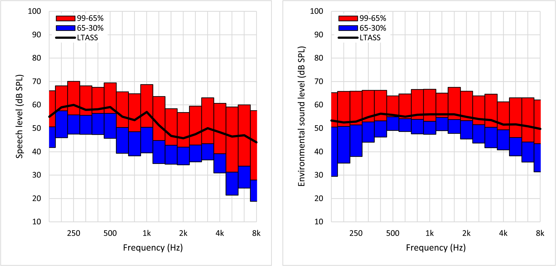
Level frequency diagrams for the speech (left panel) and environmental-sound (right panel) signals, based on short-time level percentile analysis (see text for details). Shown are long-term average spectra (black lines), 30th percentiles (lower border of blue boxes), 65th percentiles (border between red and blue boxes), and 99th percentiles (upper border of red boxes). The dynamic range within each frequency band is denoted by the difference between the 99th and 30th percentile (the combined height of a blue and red box).
The relative similarity between the long-term spectra for the speech and environmental sounds (black lines in Fig. 5) is consistent with the similar levels of audibility found in the SII analysis, which supports the premise that the differential effect of hearing loss on speech recognition versus ESR is not due to audibility differences. However, Fig. 5 shows that the two signal types differ in terms of their stationarity. Across the 18 1/3-octave bands displayed in Fig. 5, the speech has a mean dynamic range of 26.8 dB, and the environmental sounds have a mean dynamic range of 22.7 dB, amounting to a difference of 4.1 dB. Further, in several frequency bands important for speech recognition, such as 1000 Hz, the dynamic range of speech exceeds that of the environmental sounds by approximately 10 dB.
The differential fluctuation magnitudes of the two signals (where speech was found to fluctuate more than environmental sounds) cause the tasks in Experiment 1 to essentially involve: (1) recognizing a more fluctuating signal (speech) in a more stationary masker (environmental sound) and (2) recognize a more stationary signal (environmental sound) in a more fluctuating masker (speech). Because of their reduced fluctuating masker benefit compared to the NH listeners, the HI listeners may have been at a larger disadvantage for task (2) than they were for task (1).
Experiment 2
As with Experiment 1, Experiment 2 involved recognizing speech in the presence of competing environmental sounds and vice versa in order to establish the range of SBRs where both tasks are possible. In Experiment 2, however, listeners performed the speech recognition and ESR tasks separately rather than simultaneously. The primary purpose of this experiment was to compare human performance on these tasks across environmental sound types. Experiment 2 used the same speech and environmental sound signals as Experiment 1, but with more trials, which permitted the analysis of inter-environmental-sound performance differences in a way that was not possible in Experiment 1, where there was an insufficient number of trials per sound. Additionally, a secondary purpose of Experiment 2 was to allow comparison of performance across conditions of selective vs. divided attention.
MATERIALS AND METHODS
Subjects
A group of 20 young adult listeners with NH participated in Experiment 2. They all had pure-tone thresholds of 20 dB HL or better at octave frequencies from 250 to 8000 Hz (ANSI 2010), with the exception of 1 listener with a measured threshold of 25 dB HL at 250 Hz in one ear. These NH subjects were also recruited from and received credit in undergraduate courses at The Ohio State University. Their ages ranged from 18 to 26 years (mean = 19), and all were female. Young listeners with NH were selected for Experiment 2 because the goal was to establish the basic performance differences between environmental sounds and between divided and selective attention in the current task, without additional possible factors associated with aging and/or hearing loss. These listeners were distinct from those who participated in Experiment 1, and none of them had any prior exposure to the sentence materials employed in this experiment. Again, all participants gave informed consent to participate, and all procedures were approved by the IRB.
Stimuli
As in Experiment 1, stimuli for Experiment 2 consisted of sentences drawn from the standard recording of the HINT, each of which was mixed with an environmental sound that was randomly selected from the same set of 25 sounds used in Experiment 1. A set of 110 HINT sentences was used for the speech-recognition task, and a separate set of 110 HINT sentences was used for the ESR task. For each task, stimuli were mixed at 11 SBRs. The SBRs used in the speech-recognition task were −35, −30, −25, −20, −15, −10, −5, 0, 5, 10, and 15 dB. The SBRs used in the ESR task were 0, 7, 14, 21, 28, 35, 42, 49, 56, 63, and 70 dB. Unlike Experiment 1, participants only completed one task at a time in Experiment 2. For this reason, it was not necessary to test at SBRs that lay well beyond the threshold for ceiling performance for one task in order to accommodate non-ceiling portions of the psychometric function for the other task. For this reason, narrower ranges of SBRs, different from those used in Experiment 1, were used for each task here. Other than the SBRs employed, the process for mixing and scaling the stimuli was the same as in Experiment 1.
Procedure
The same general procedures that were used in Experiment 1 were followed in Experiment 2, unless otherwise noted. Listeners were tested in a single session consisting of an ESR task followed by a speech-recognition task.
ESR Task.
Listeners heard 330 stimuli in the ESR task, blocked by SBR, with 10 trials per block. For each of the 11 SBRs, there were 3 blocks of 10 stimuli each. These 33 SBR blocks were presented in a random order for each listener. The same set of 110 HINT sentences was repeated 3 times in the experiment, with sentences presented in the same order each time. The repetition of sentences was allowed because the task only involved ESR and not sentence recognition. Listeners were instructed to attend to the background sound, click on the corresponding labeled picture, and guess if unsure. As in Experiment 1, the playback sequence of each stimulus was triggered by the listener’s response to the previous one.
Before to formal testing, listeners were familiarized with the 25 environmental sounds, as described in Experiment 1. They also practiced identifying sounds in the presence of competing speech using 11 stimuli mixed at SBRs of 6, 10, 14, 18, 22, 26, 40, 44, 48, 52, and 56 dB, with difficulty of the task increasing with each successive practice trial (environmental sounds are less audible at higher SBRs). The sentences used during familiarization were distinct from those used for formal testing. After completing all experimental trials for the ESR task, listeners next performed the speech-recognition portion of the experiment.
Speech-recognition task.
For the speech-recognition task, listeners heard 110 stimuli and were instructed to attend to the talker’s voice and repeat back each sentence as best as they could, guessing if unsure. The sentences were blocked by SBR, with 10 sentences per block, and the SBR blocks were presented in random order for each subject. The experimenter controlled the stimulus presentation and recorded the number of words correctly reported by the listener in each trial.
Before to formal testing, listeners practiced recognizing speech in the presence of randomly selected background sounds using 11 sentences mixed at 16, 12, 8, 4, 0, −4, −8, −12, −16, −20, and −24 dB SBR, with speech recognition becoming more difficult with each successive practice trial. Again, the sentences used in familiarization were not used during formal testing. Experiment 2 lasted approximately one hour for each participant, including familiarization.
RESULTS
Figure 6 displays normalized psychometric functions for speech recognition and ESR based on the performance of the 20 NH listeners. Psychometric functions were fitted using the same linking function, software, and other parameters outlined in Experiment 1.
Fig. 6.
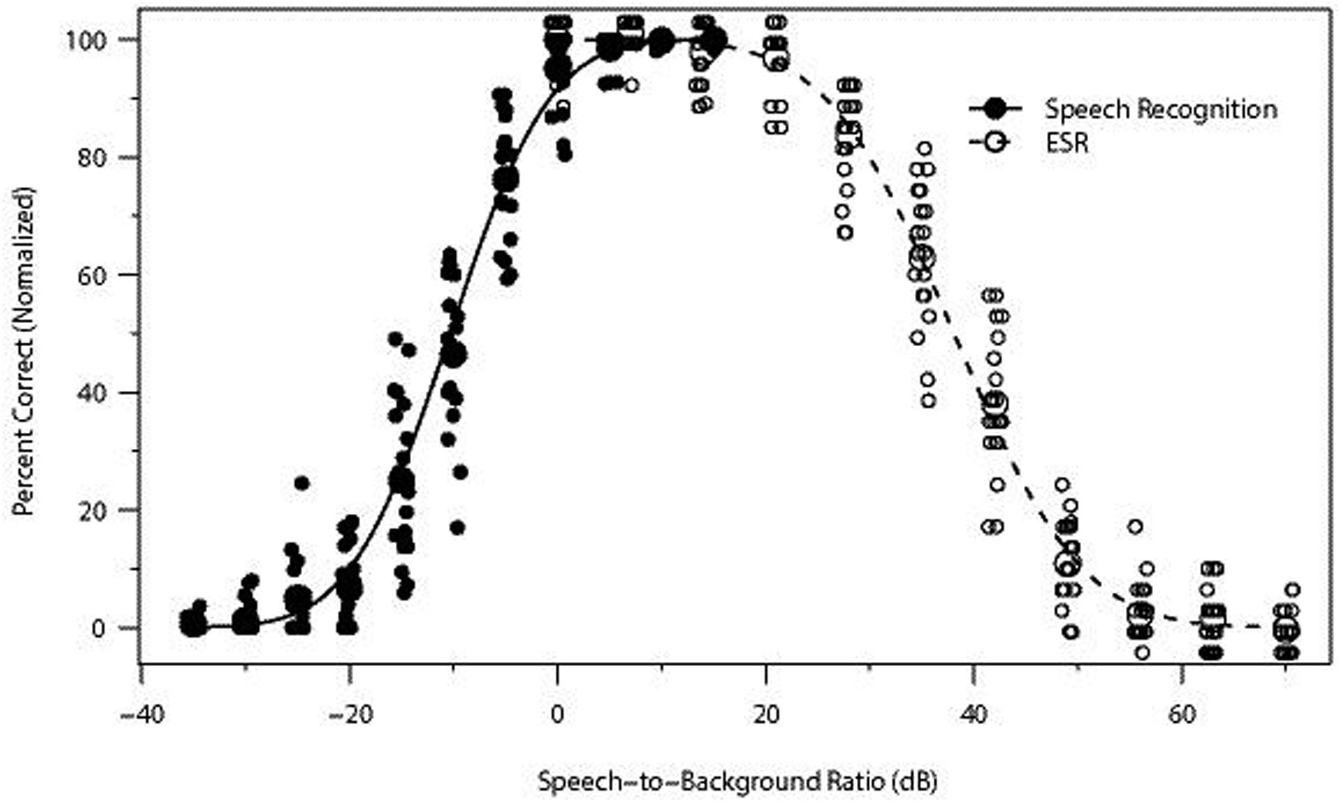
As Fig. 3, but for the 20 normal-hearing subjects who performed the selective attention task in Experiment 2.
For speech recognition, performance was near perfect when the SBR was sufficiently high, with an estimated lapse rate of less than 0.01% (asymptote at 99.99% correct). Combined with a guess rate of 0%, normalization had a negligible effect on the psychometric function for recognition. The normalized threshold for 50% HINT words correct was −10.4 dB SBR (95% CI [−10.6, −10.1]), and the normalized 95% threshold was 2.0 dB SBR (95% CI [1.5, 2.5]).
The lapse rate for ESR was estimated to be 2.7% (95% CI [2%, 3.5%]), indicating that unnormalized performance plateaued at 97.3% correct. The normalized 50% and 95% correct thresholds were 38.1 (95% CI, [37.7, 38.5]) and 22.2 (95% CI, [21.3, 23.3]) dB SBR, respectively.
The estimated distance between the normalized 50% correct threshold for speech recognition and that for ESR was 48.5 dB. This distance was 24.2 dB between the 2 thresholds for 95% correct. The optimal SBR for maximizing both speech recognition and ESR, defined as the intersection between the 2 normalized psychometric functions, was 10.8 dB, at which point normalized performance was 99.8% correct for both tasks (unnormalized speech recognition = 99.7 % correct; unnormalized ESR = 97.1% correct).
Figure 7 displays normalized psychometric functions for speech recognition and ESR for each individual environmental sound stimulus used in this study. The repetition of sentences in Experiment 2 produced a number of trials sufficient to allow this analysis of individual environmental sounds. The symbols and fit lines are as in Figs. 3, 4, and 6. Panels are arranged in order of decreasing range between normalized 50% correct thresholds for speech recognition and ESR. For each environmental sound and task type, the lapse rate was modeled as a free parameter unless accuracy was 100% at the 3 highest SBRs for speech recognition or the 3 lowest SBRs for ESR, in which case the lapse rate was set to 0%. The lapse rate was also set to 0% if a negative value was calculated. The guess rate was set to 0% for speech recognition and to 4% for ESR. All other relevant fitting procedures and parameters are described in Experiment 1.
Fig. 7.
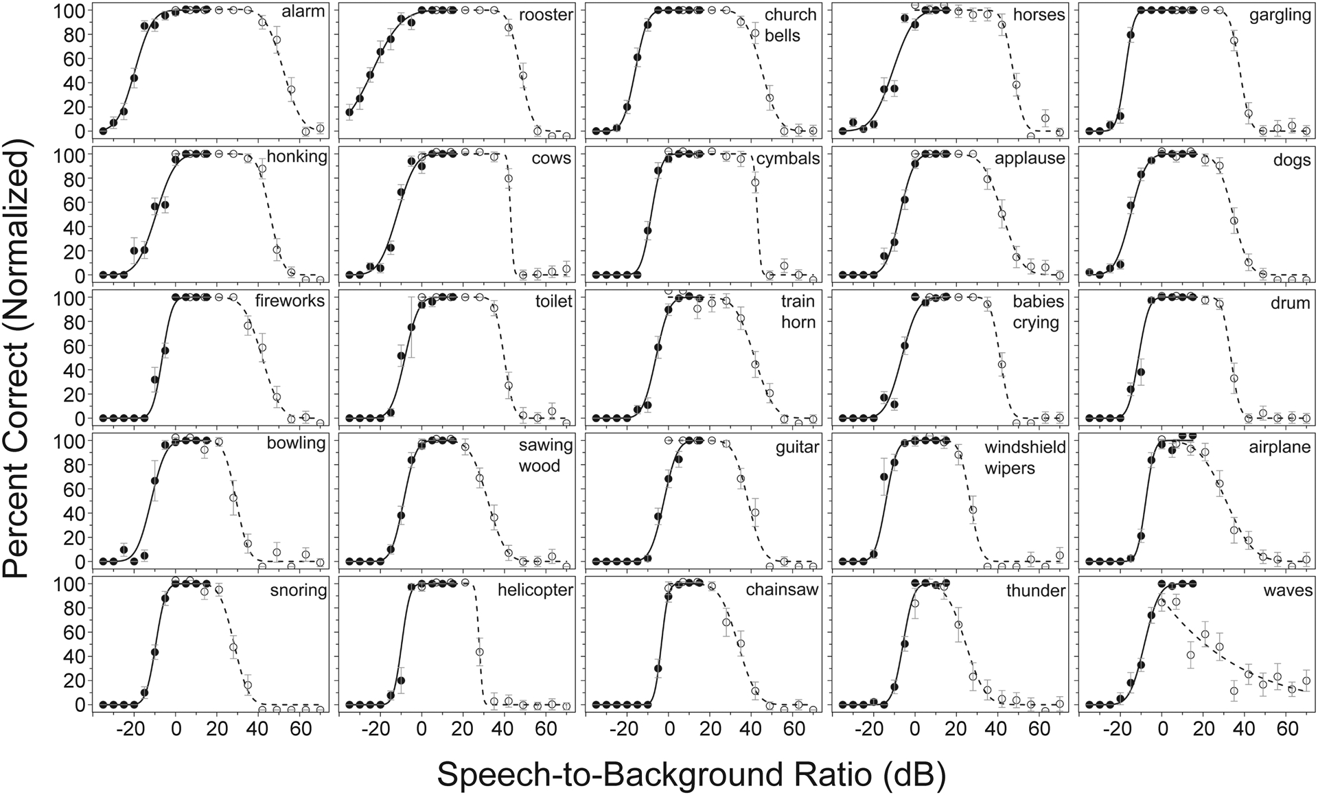
Psychometric functions for speech recognition and environmental sound recognition for 25 environmental background sounds. Each panel represents data from a different environmental sound, indicated by the label in the top right corner of the panel. As in other figures, solid black circles and lines denote speech recognition whereas open circles and dashed lines represent environmental sound recognition. Error bars indicate the standard error of the mean.
With the exception of “waves,”2 lapse rates varied from 0% to 4.9%, indicating that the effect of normalization was modest for the curves in Fig. 7. For each environmental sound, if the two psychometric functions crossed at a single point, the optimal SBR for maximizing both speech recognition and ESR was calculated as the point of intersection. If both psychometric functions plateaued at 100% correct (normalized) and overlapped over a range of SBRs, then the optimal SBR value was calculated as the midpoint in dB between normalized 50% correct thresholds.
Apparent in Fig. 7 is that all environmental sounds could be reliably identified (with one exception, “waves”). Also apparent is that the range of SBRs over which speech recognition and ESR both remain near ceiling is considerable for the large majority of environmental sounds. With regard to the exception, it appears that listeners tended to guess “waves” by default when they were unable to hear the target environmental sound.3
Table 1 contains a confusion matrix for selective-attention ESR. Stimulus sounds are listed vertically in the first column, and subject responses are listed horizontally in the first row of the table, both in alphabetical order. Each cell indicates the number of responses given to each stimulus type summed across SBRs and listeners. The total number of presentations of each stimulus and listener responses of each stimulus are given in the last column and row, respectively. There were between 217 and 297 total presentations of each stimulus type (M = 264, SD = 17.2). Even though the number of presentations for “waves” (277) was near the mean, the number of “waves” responses (805) was 4.4 standard deviations above the mean number of responses (264), indicating a listener bias for this response.
Table 1:
Confusion matrix for environmental sound recognition in the presence of competing speech and under conditions of selective attention. Stimuli presented are listed in the first column, and listener responses are shown in the first row. The number in each cell represents the number of listener responses given to each environmental sound stimulus across all SBRs.
| Response Stimulus | airplane | alarm | applause | babies crying | bowling | chainsaw | church bells | cows | cymbals | dogs | drum | fireworks | gargling | guitar | helicopter | honking | horses | rooster | sawing wood | snoring | thunder | toilet | train horn | waves | windshield wipers | Total |
|---|---|---|---|---|---|---|---|---|---|---|---|---|---|---|---|---|---|---|---|---|---|---|---|---|---|---|
| airplane | 121 | 2 | 13 | 1 | 5 | 5 | 4 | 2 | 1 | 6 | 9 | 2 | 5 | 8 | 4 | 8 | 4 | 3 | 6 | 4 | 3 | 32 | 5 | 253 | ||
| alarm | 1 | 181 | 3 | 1 | 1 | 1 | 2 | 4 | 4 | 1 | 6 | 4 | 2 | 4 | 1 | 1 | 1 | 7 | 1 | 4 | 4 | 1 | 21 | 256 | ||
| applause | 2 | 1 | 157 | 2 | 1 | 7 | 3 | 2 | 1 | 6 | 5 | 3 | 2 | 1 | 3 | 2 | 2 | 5 | 2 | 10 | 4 | 4 | 36 | 4 | 265 | |
| babies crying | 6 | 2 | 5 | 162 | 2 | 5 | 1 | 5 | 2 | 1 | 3 | 4 | 4 | 8 | 3 | 1 | 4 | 2 | 7 | 1 | 5 | 3 | 2 | 21 | 2 | 261 |
| bowling | 2 | 3 | 6 | 118 | 1 | 4 | 6 | 3 | 5 | 12 | 2 | 8 | 3 | 3 | 3 | 2 | 14 | 3 | 11 | 6 | 4 | 34 | 7 | 260 | ||
| chainsaw | 2 | 8 | 1 | 3 | 120 | 4 | 4 | 4 | 6 | 3 | 3 | 11 | 3 | 2 | 6 | 5 | 18 | 1 | 9 | 8 | 1 | 28 | 8 | 258 | ||
| church bells | 6 | 1 | 1 | 180 | 8 | 2 | 2 | 6 | 7 | 1 | 1 | 4 | 3 | 5 | 1 | 12 | 2 | 3 | 18 | 4 | 267 | |||||
| cows | 3 | 2 | 5 | 1 | 2 | 2 | 156 | 1 | 1 | 4 | 3 | 1 | 6 | 3 | 3 | 7 | 5 | 12 | 1 | 3 | 2 | 24 | 7 | 254 | ||
| cymbals | 3 | 1 | 4 | 1 | 2 | 3 | 4 | 4 | 167 | 1 | 7 | 5 | 2 | 3 | 3 | 7 | 7 | 1 | 3 | 4 | 3 | 33 | 6 | 274 | ||
| dogs | 3 | 4 | 10 | 2 | 6 | 6 | 3 | 139 | 5 | 4 | 7 | 2 | 7 | 2 | 6 | 7 | 13 | 2 | 3 | 5 | 24 | 8 | 268 | |||
| drum | 1 | 2 | 6 | 1 | 4 | 1 | 3 | 3 | 5 | 4 | 136 | 10 | 1 | 9 | 3 | 5 | 7 | 11 | 8 | 5 | 7 | 30 | 4 | 266 | ||
| fireworks | 4 | 2 | 7 | 3 | 2 | 1 | 2 | 5 | 2 | 6 | 160 | 3 | 5 | 2 | 2 | 6 | 4 | 8 | 1 | 5 | 3 | 2 | 29 | 2 | 266 | |
| gargling | 2 | 1 | 5 | 3 | 6 | 2 | 2 | 6 | 4 | 2 | 7 | 155 | 4 | 5 | 2 | 6 | 4 | 9 | 6 | 24 | 3 | 258 | ||||
| guitar | 5 | 1 | 8 | 2 | 3 | 8 | 3 | 3 | 3 | 4 | 4 | 4 | 167 | 3 | 3 | 4 | 2 | 12 | 2 | 7 | 7 | 5 | 34 | 3 | 297 | |
| helicopter | 2 | 3 | 14 | 2 | 4 | 3 | 3 | 6 | 1 | 4 | 3 | 7 | 7 | 2 | 107 | 2 | 4 | 4 | 11 | 3 | 9 | 10 | 3 | 50 | 5 | 269 |
| honking | 1 | 7 | 3 | 2 | 4 | 7 | 2 | 5 | 6 | 5 | 4 | 4 | 182 | 1 | 4 | 6 | 5 | 4 | 25 | 8 | 285 | |||||
| horses | 2 | 1 | 1 | 2 | 3 | 1 | 7 | 6 | 2 | 7 | 2 | 5 | 3 | 2 | 5 | 184 | 9 | 2 | 1 | 11 | 4 | 3 | 20 | 3 | 286 | |
| rooster | 3 | 2 | 2 | 5 | 2 | 1 | 1 | 2 | 1 | 4 | 5 | 5 | 1 | 2 | 5 | 185 | 2 | 6 | 4 | 4 | 13 | 3 | 258 | |||
| sawing wood | 2 | 1 | 8 | 1 | 5 | 4 | 4 | 6 | 5 | 6 | 2 | 3 | 4 | 3 | 4 | 6 | 17 | 4 | 137 | 3 | 8 | 6 | 33 | 4 | 276 | |
| snoring | 3 | 1 | 9 | 1 | 3 | 5 | 4 | 2 | 7 | 2 | 9 | 8 | 5 | 4 | 3 | 4 | 5 | 4 | 19 | 97 | 11 | 4 | 1 | 37 | 6 | 254 |
| thunder | 5 | 2 | 10 | 8 | 4 | 2 | 5 | 1 | 3 | 4 | 19 | 5 | 5 | 8 | 6 | 8 | 3 | 90 | 13 | 3 | 53 | 11 | 268 | |||
| toilet | 1 | 2 | 3 | 1 | 5 | 4 | 3 | 6 | 2 | 7 | 4 | 5 | 2 | 4 | 2 | 7 | 9 | 138 | 3 | 16 | 1 | 225 | ||||
| train horn | 3 | 1 | 5 | 3 | 3 | 4 | 2 | 1 | 2 | 1 | 3 | 5 | 2 | 3 | 2 | 27 | 8 | 6 | 3 | 5 | 2 | 156 | 31 | 4 | 282 | |
| waves | 7 | 7 | 1 | 5 | 3 | 5 | 2 | 2 | 4 | 6 | 5 | 4 | 6 | 12 | 4 | 4 | 5 | 9 | 5 | 44 | 9 | 2 | 114 | 12 | 277 | |
| windshield wipers | 2 | 2 | 8 | 2 | 4 | 5 | 6 | 2 | 1 | 6 | 5 | 7 | 4 | 4 | 1 | 4 | 4 | 20 | 1 | 7 | 7 | 1 | 25 | 89 | 217 | |
| Total | 183 | 214 | 311 | 186 | 194 | 195 | 256 | 242 | 248 | 191 | 247 | 307 | 252 | 266 | 201 | 266 | 294 | 279 | 353 | 128 | 296 | 260 | 217 | 805 | 209 | 6600 |
Table 2 lists optimal SBR values, normalized 50% and 95% correct thresholds for speech recognition and ESR, and ranges between these thresholds for each of the 25 environmental sounds. Sounds are listed in descending order of distance between normalized 50% correct thresholds. Because the sound “waves” is so clearly an outlier, it has been excluded from the descriptive statistics reported below. Thresholds for normalized 50% correct speech recognition ranged from −23.8 dB SBR for “rooster” to −2.2 dB SBR for “guitar,” with a mean of −10.5 (SD = 5.1). Thresholds for normalized 50% correct ESR ranged from 24.6 dB SBR for “thunder” to 52.2 dB SBR for “alarm,” with a mean of 37.9 (SD = 7.6). Again, for ESR, lower SBR thresholds represent poorer recognizability, and higher SBR thresholds represent better recognizability. Fifty-percent-correct thresholds for speech recognition and ESR appeared to be weakly inversely related, but the Pearson’s correlation coefficient was not significant [r(23) = −0.32, p = 0.12]. Normalized thresholds for 95% speech recognition ranged from −12.2 dB SBR for “gargling” to 6.2 dB SBR for “guitar” (M = −2.0, SD = 4.5). Thresholds for 95% ESR accuracy were as low as −20.7 dB SBR for “sawing wood” and as high as 41.7 dB SBR for “train horn” (M = 32.2, SD = 6.6). Since a train horn may be a highly relevant sound for personal safety, its high recognizability at even low levels relative to concurrent speech is encouraging.
Table 2:
Optimal SBR values, normalized 50%- and 95%-correct thresholds for speech recognition and ESR, and ranges between these thresholds for each of the 25 environmental sounds. The values for “waves” were calculated based on the unnormalized ESR function for this sound due to its irregular form.
| Stimulus Name | Optimal SBR (dB) | 50%-Correct Threshold for Speech Recognition (dB SBR) | 50%-Correct threshold for Environmental Sound Recognition (dB SBR) | Range between 50%-Correct thresholds (dB) | 95%-Correct Threshold for Speech Recognition (dB SBR) | 95%-Correct threshold for Environmental Sound Recognition (dB SBR) | Range between 95%-Correct thresholds (dB) |
|---|---|---|---|---|---|---|---|
| Alarm | 16.3 | −19.6 | 52.2 | 71.8 | −8.6 | 41.1 | 49.7 |
| Rooster | 12.0 | −23.8 | 47.7 | 71.5 | −5.7 | 40.0 | 45.7 |
| Church Bells | 14.5 | −16.0 | 45.1 | 61.2 | −8.4 | 34.4 | 42.8 |
| Horses | 18.3 | −10.8 | 47.4 | 58.1 | 2.5 | 40.7 | 38.2 |
| Gargling | 10.1 | −17.6 | 37.8 | 55.4 | −12.2 | 31.5 | 43.7 |
| Honking | 18.2 | −9.4 | 45.7 | 55.1 | 2.6 | 37.7 | 35.0 |
| Cows | 15.5 | −11.9 | 42.9 | 54.8 | −0.8 | 41.1 | 41.9 |
| Cymbals | 17.3 | −8.3 | 43.0 | 51.3 | −1.8 | 40.7 | 42.6 |
| Applause | 17.4 | −7.4 | 42.2 | 49.6 | 1.5 | 30.0 | 28.5 |
| Dogs | 9.7 | −15.0 | 34.5 | 49.5 | −5.2 | 24.5 | 29.7 |
| Fireworks | 17.8 | −6.4 | 41.9 | 48.3 | −0.2 | 30.4 | 30.6 |
| Toilet | 15.8 | −8.2 | 39.8 | 48.0 | 0.4 | 33.9 | 33.4 |
| Train Horn | 13.3 | −6.1 | 41.7 | 47.7 | 2.2 | 41.7 | 39.4 |
| Babies Crying | 17.3 | −6.5 | 41.1 | 47.6 | 3.7 | 35.0 | 31.2 |
| Drum | 11.1 | −11.2 | 33.4 | 44.7 | −4.8 | 27.8 | 32.6 |
| Bowling | 8.8 | −11.8 | 29.4 | 41.2 | −2.6 | 21.6 | 24.2 |
| Sawing Wood | 11.6 | −8.8 | 32.0 | 40.8 | −1.1 | 20.7 | 21.8 |
| Windshield Wipers | 6.5 | −14.1 | 26.6 | 40.7 | −7.3 | 26.6 | 33.9 |
| Guitar | 18.1 | −2.2 | 38.5 | 40.7 | 6.2 | 29.3 | 23.1 |
| Airplane | 1.5 | −7.7 | 31.1 | 38.9 | −2.4 | 31.1 | 33.5 |
| Snoring | 9.4 | −9.6 | 28.4 | 37.9 | −3.3 | 28.4 | 31.7 |
| Helicopter | 9.0 | −9.7 | 27.8 | 37.5 | −4.6 | 25.5 | 30.1 |
| Chainsaw | 6.7 | −3.4 | 33.7 | 37.1 | 0.9 | 33.7 | 32.7 |
| Thunder | 4.8 | −5.9 | 24.6 | 30.4 | 0.8 | 24.6 | 23.7 |
| Waves | −1.2 | −8.4 | 21.0 | 29.4 | 0.9 | −3.2 | −2.3 |
| Mean | 12.0 | −10.4 | 37.2 | 47.6 | −1.9 | 31.7 | 33.6 |
| Standard Deviation | 5.5 | 5.0 | 8.2 | 10.9 | 4.4 | 6.8 | 7.9 |
Optimal SBRs for balancing speech recognition with ESR for different environmental sounds also varied, ranging from 1.5 dB for “airplane” to 18.3 dB for “horses,” (M = 12.5, SD = 4.8), indicating that the optimal SBR value depends somewhat on the type of environmental sound present. But perhaps more importantly, all sounds had a considerable range between normalized 50%-correct thresholds, from 30.4 dB for “thunder” to 71.8 dB for “alarm.” The ranges between normalized 95% correct thresholds for speech recognition and ESR varied from 21.8 (“sawing wood”) to 49.7 dB (“alarm”), indicating that these environmental sounds possessed a range over which both speech recognition and ESR could be essentially maximized. Further, these ranges overlapped for all of the sounds except for the outlier “waves,” suggesting some degree of commonality across the ranges for different sounds. Figure 8 displays normalized 95%-correct thresholds for speech recognition (filled circles), ESR (open circles), and optimal SBRs (X’s) for each of the 25 environmental sounds. The shaded region indicates the span (14.5 dB) over which ranges overlap across all sounds except for “waves” (The two psychometric functions for “waves” intersected at 90% correct, meaning there was no range of SBRs over which speech recognition and ESR exceeded 95% correct for this sound).
Fig. 8.
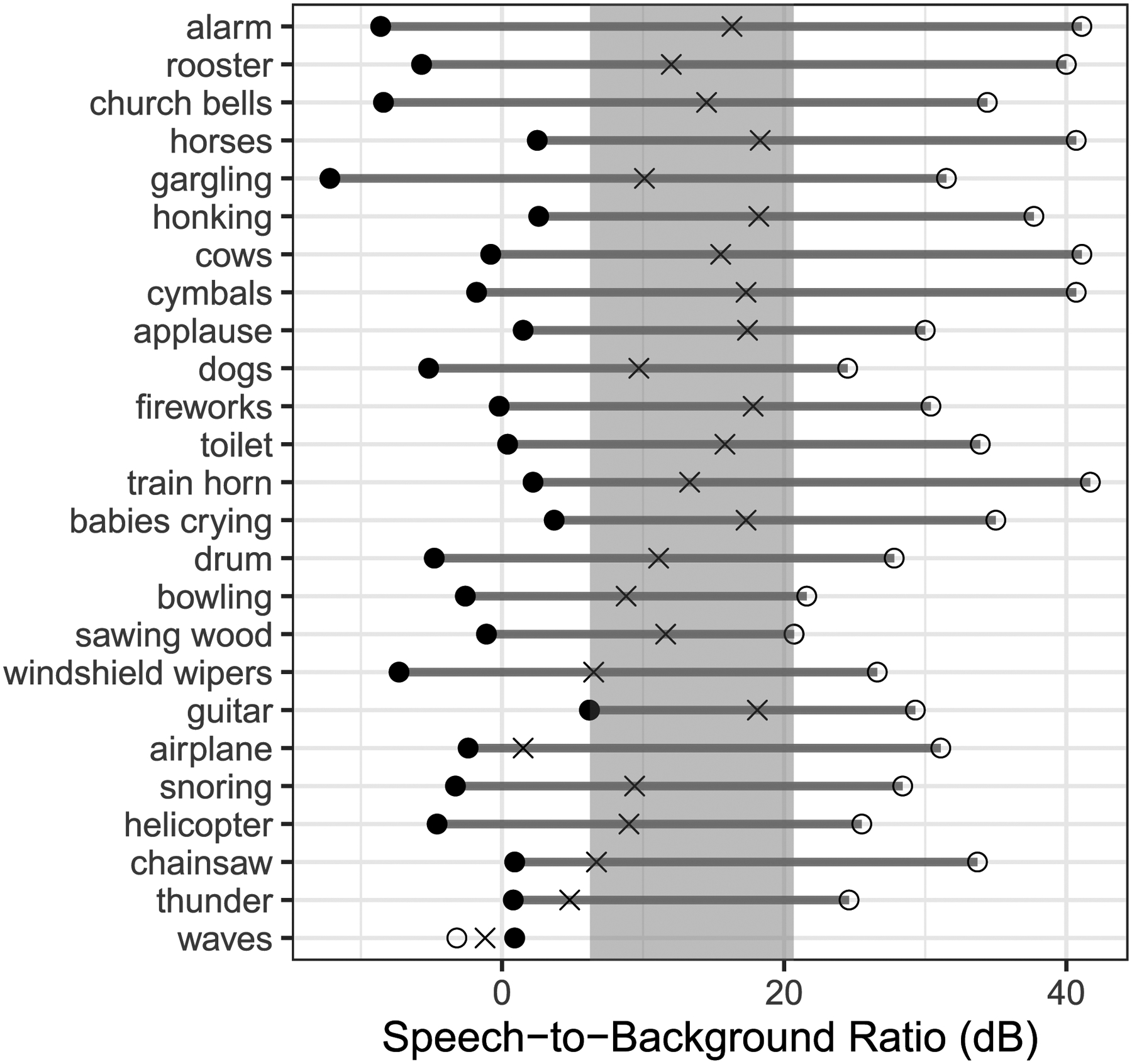
Range plot of normalized 95%-correct thresholds for 25 environmental background sounds. Thresholds for recognition and environmental sound recognition are denoted by filled and open circles, respectively. The shaded area indicates the range of speech-to-background ratios where performance is at least 95% correct on both tasks for all sounds (except for “waves”).
The secondary question addressed in Experiment 2 involves the effect of selective vs. divided attention for NH listeners performing the mixed tasks of speech recognition and ESR. The overall 50%-correct threshold for selective-attention speech recognition was −10.4 dB SBR, compared to −10.7 dB SBR for divided attention in Experiment 1, a difference of 0.3 dB. For ESR, the overall normalized thresholds for 50% correct were 38.1 and 36.7 dB for selective and divided attention, respectively, amounting to a difference of 1.4 dB. These values are identical out to three decimal places regardless of whether or not normalized or unnormalized values are used.
Mixed-effects logistic models were constructed to test the effect of selective vs. divided attention on speech recognition and ESR for NH listeners using the same software and packages cited in Experiment 1. In the first model (speech recognition), the outcome variable was binary data for words correct (n = 26,109 observations), and the fixed effects were SBR (dB), attention type (deviation coded: selective = 0.5, divided = −0.5), and their two-way interaction. This model included random intercepts for listener. Models for speech recognition that included random intercepts or slopes for sentence and/or and environmental sound failed to converge.
In the second model (ESR), the outcome variable was binary data for environmental sounds correct (n = 9,350 observations). This model also had fixed effects for SBR (dB), attention type, and their two-way interaction. Attention type was coded in the same way as in the other model. The model for ESR included random intercepts for sentence, listener, and environmental sound. Models that specified random slopes failed to converge.
As expected, the effect of SBR was large and significant in both of these models. Larger SBRs resulted in higher predicted speech recognition (β = 0.22, SE = 0.003, z = 64.6, p < 0.001) and lower ESR performance (β = −0.14, SE = 0.003, z = −44.5, p < 0.001). The main effect of attention type was also significant for both speech recognition (β = 0.58, SE = 0.16, z = 3.73, p < 0.001) and ESR (β = 2.0, SE = 0.23, z = 8.64, p < 0.001). Although the magnitude of the performance difference between selective and divided attention was very small (with selective attention resulting in slightly higher performance), it was statistically significant likely due to the power associated with the large number of observations. The interaction between SBR and attention type was also significant in both models. For speech recognition, the effect of selective attention was greater at higher SBRs (β = 0.061, SE = 0.007, z = 8.91, p < 0.001) whereas for ESR, the effect of selective attention was greater at lower SBRs (β = −0.052, SE = 0.005, z = −10.2, p < 0.001).
DISCUSSION
The results of these experiments illustrate the trade-off that exists between speech recognition and ESR when the amplitude relationship between the two (SBR) is varied. They also demonstrate that it is possible to find a balance between these two competing aims – good speech recognition and good recognition of environmental sounds – by selecting an SBR where performance is high for both tasks.
The results of Experiments 1 and 2 demonstrate that, when speech and environmental sounds are presented at the same level, i.e., 0 dB SBR, recognition is higher for environmental sounds than for speech. These findings indicate that, although there is mutual masking between the environmental sounds and speech, the environmental sounds tend to be more effective maskers of speech than the converse. Several factors may account for this asymmetry in masking between the two types of signals, including the fact that speech recognition is an open-set task whereas the ESR task was closed set, as well as the fact that the environmental sounds are more stationary whereas the speech signals possess fluctuations that render them less effective maskers.
It was found that both NH and HI listeners are capable of simultaneously high speech recognition and high ESR over a range of SBRs. As Figs. 3 and 6 show, NH listeners display near-ceiling levels of performance for speech recognition and ESR over a range of 20 dB or more. This range was similar in Exps. 1 and 2 where different tasks were employed. The center points, representing the single optimal tradeoff between speech recognition and ESR, were 12.2 and 10.8 dB SBR, at which normalized performance on both tasks was over 99% correct. Performance on both tasks remained over 95% correct (normalized) from 2 or 3 dB to 22 dB SBR. This large range over which NH listeners can do both tasks very well may be partially due to the differing natures of the two tasks. In contrast with speech perception, which involves recognizing and interpreting linguistic units that follow specific rules and patterns of a given language, environmental sounds may be labeled often with a single word. Further, and unlike sentences, environmental sounds can typically be identified from a single brief glimpse. These aspects may facilitate environmental sound recognition and its segregation from speech.
The SBR value representing optimal concurrent performance was roughly 6 dB lower for HI listeners (value = 5.1 dB SBR, performance on both tasks over 96% correct normalized). Further, the range was smaller for these listeners – unlike the broad range over which NH listeners displayed near-ceiling performance, 95%-plus normalized performance on both tasks occurred from only 4.7 to 5.8 dB for the HI listeners. The lower optimal SBR and smaller SBR range of high concurrent performance for the HI listeners were primarily the result of the larger effect of hearing loss on ESR relative to the effect of hearing loss on speech recognition. The results of the SII-based audibility analysis indicate that this effect was not caused by a lack of audibility for the environmental sounds. Rather, the short-time level percentile analysis indicated that a more likely explanation involves the reduced fluctuating masker benefit for HI listeners. Several bases for reduced fluctuating masker benefit have been proposed, including audibility limitations during the silent gaps of the masker (George et al. 2006), susceptibility to forward masking for high-rate masker modulations (Jensen & Bernstein 2019), and cognitive effects associated with aging (Dubno et al. 2003). Although the present study was not designed to clarify these possible bases, the results are consistent with previous reports of reduced fluctuating masker benefit for HI listeners.
In spite of the poorer relative performance shown by the HI group, particularly on the ESR task, there were several encouraging results: (i) the 50% normalized correct range for the HI listeners was very broad (30.9 dB), (ii) the optimal SBR for HI listeners also yielded high performance for NH listeners in the same Experiment (HI optimal SBR falls within the NH 95%-correct SBR range), and (iii) the optimal NH SBR yields excellent speech recognition (above 99% correct normalized) for HI listeners while still providing for good ESR (approximately 86% correct normalized).
The conversation thus far has largely assumed that speech recognition and ESR are to be jointly optimized at equal importance. But a variety of other scenarios can be envisioned. For example, the relatively narrow range over which HI performance is jointly above 95% correct can be addressed by emphasizing near-perfect speech recognition but acknowledging that recognition of environmental sounds at less-than-perfect levels can still occur. An example of this approach was provided above where it was indicated that shifting the ideal SBR for HI listeners roughly 6 dB by using the optimal value for NH, still yields 99% normalized HI speech recognition and 86% normalized HI ESR (99% and 85% unnormalized).
Different sounds can interact differently with speech. The alarm used in this study, for example, displayed a vast range (49.7 dB) over which normalized speech recognition and ESR are both above 95%. This may be a particularly useful quality of an alarm sound: it is easily audible and identifiable in the presence of a competing speech signal without unduly disrupting the transmission of speech information. For other sounds, such as “sawing wood,” this range is less than half as wide (21.8 dB), suggesting greater auditory interference between the speech and “sawing wood” signals. The observed differences in the amount of interference between speech and different environmental sounds may be due to a combination of factors such as the degree of spectral overlap between the two signal types, the likelihood of confusion between different environmental sound alternatives, and the differential recognizability of environmental sounds based on a small number of short glimpses. Despite these differences, there is a substantial degree of commonality across the 95%-correct ranges for the environmental sounds employed in this study. With the exception of “waves,” all of the environmental sounds allowed for normalized speech recognition and ESR scores of at least 95% between 6.2 and 20.7 dB SBR, a range of 14.5 dB (see Fig. 8). This span therefore represents an essentially optimal SBR range for a wide variety of continuous environmental sounds for NH listeners. Furthermore, for 22 of these 24 sounds, the optimal SBR fell within this range. For the two sounds whose optimal SBRs fell outside this range (“airplane” and “thunder”) the psychometric function for ESR was considerably less steep than the function for speech recognition, leading the functions to intersect at relatively low SBRs within each sound’s 95%-threshold ranges. In light of the broadly similar ranges between 95%-correct thresholds across sounds, it is apparent that many different types of continuous environmental sounds interact with speech in similar ways.
The present study involved two tasks designed to differ in the amount and type of attention involved: the theoretical endpoints of fully divided and fully selective attention. Thus, these results show the largest drop in performance that is likely to arise from the manipulation of attention when the tasks are speech recognition and ESR. Divided attention resulted in slightly poorer performance for NH listeners on both the speech recognition and ESR tasks. Although reliable and highly significant in the statistical models, these drops in performance were very small in magnitude (0.3-dB threshold shift for speech recognition and 1.4-dB threshold shift for ESR). Accordingly, the results obtained with regard to balancing speech recognition and ESR do not appear to be largely affected by the exact task that the listener is asked to perform or its associated demands, at least for NH listeners.
It should be emphasized that the current initial examination of attention involved only young NH listeners. A proper examination in HI listeners would require the consideration of various factors not addressed currently, including subject age and the various components of cognitive status (e.g., working memory). The detrimental impact of divided attention might be expected to be larger in typical (older) listeners with hearing loss than in young NH individuals. Accordingly, the results of Experiment 1 likely represent a worst-case scenario for HI listeners (because divided attention was addressed), and better access to environmental sounds concurrent with speech might be anticipated if the listening demands are changed.
Because the present study represents an initial examination of the current effect, it was designed with intentionality to address the simplest of questions: does a range of SBRs exist over which both speech recognition and ESR are both high? The results are highly encouraging because the simple answer is yes. But as with any initial study, the current one has limitations. The attention aspects addressed above are one example. Also, co-located sounds were used in order to simulate a worst-case situation. But when sound sources are separated spatially, as is often the case in realistic conditions, the range of SBRs where performance is high for both speech recognition and ESR may be expanded due to spatial release from masking (Bregman 1990), which was not examined in the present study. Any spatial release from masking would also likely be tempered by room reverberation (Kidd et al. 2005), which was likewise not addressed in the present study. And all these factors may differ for NH versus HI listeners. The decision was also made to prioritize speech recognition in Experiment 1 by having participants provide a speech-perception response first, followed by an ESR response.
As explained in the first Materials and Methods section, only sounds that were relatively continuous and had a duration similar to that of the sentences were used in this study. This was done because only such sounds have the potential to mask speech, again providing a worst-case situation. On one hand, this limits the current examination to only a subclass of environmental sounds. But on the other hand, isolated transient sounds are not good maskers of speech (Miller & Licklider 1950) or any other relatively continuous sound, and so speech recognition remains high in the presence of these transient sounds regardless of the amplitude relationship between the two. In addition to their relative lack of masking potential, transient sounds can elicit phonemic restoration of speech, which can allow good speech recognition to persist (Warren 1970; Bashford et al. 1992). The opposite question involving the recognition of low-level transient environmental sounds in the presence of competing speech remains. But as Figs. 3, 4, and 6 show, ESR and therefore presumably good environmental-sound awareness of long-duration (not transient) environmental sounds can occur even when the speech is 20 to 35 dB more intense than the environmental sound. This result is somewhat promising for the availability of (untested) shorter duration sounds across various listening situations.
Another limitation involves the generalizability of the present findings involving the current 25 environmental sound tokens. On one hand, the study of speech perception typically involves a limited number of utterances, the results of which are extrapolated to draw conclusions regarding speech in general. A similar approach was taken here, in which the results from an array of different environmental sounds were averaged to draw conclusions about environmental sounds in general. But if the acoustic characteristics of environmental sounds vary more broadly than the relatively limited array of sounds that humans are capable of producing, then the extrapolation from the current results to environmental sound in general may be more tenuous. A more specific and likely larger effect also exists: Considerable variability exists across exemplars of a particular sound type. For example, a kettle drum and a snare drum possess very different acoustic characteristics, even though both are “drum” sounds, and so they may differ with regard to the range of SBRs over which speech and ESR are both high. Therefore, even though the present findings provide a sense of the similarities and differences among various types of sounds, given exemplars of a sound type cannot be assumed to represent all tokens of that type.
High speech recognition and high ESR are two desirable outcomes in many listening situations, but several other important variables merit consideration. These include subjective listening comfort, naturalness, speech quality, and listening effort. Each of these factors affects individuals’ satisfaction and usage of hearing devices (McCormack & Fortnum 2013). Listening effort in particular should be as low as possible because high levels of listening effort lead to fatigue and reduced well-being (Alhanbali et al. 2017). Anecdotal reports from participants and experiences of the researchers during informal listening suggest that even the divided attention task in this study is fairly straightforward and surprisingly not demanding. However, additional studies will be needed to consider these various aspects.
As described in the Introduction, the issue of ESR is an overlooked but important one especially in the context of increasingly powerful noise-reduction technology. Clearly, good speech recognition is critical. But recognition of background environmental sounds is also important for the safety and comfort issues described earlier. But noise reduction based on deep learning has advanced over the past decade to the point that, at least for large laboratory-based networks not yet implemented, essentially complete removal of all sound sources except the target speech is possible. This performance will undoubtedly recede some as implementation measures are undertaken. But modern noise reduction is becoming so effective that we are approaching a point at which it can be too effective. One example of this involves the unavailability of potential warning sounds in the environment described earlier. Another involves naturalness – it would be unnatural to enter a room filled with people visibly talking yet hear only the voice of the dominant target talker in front of you.
Accordingly, the results of this study can be used to inform the design of future noise-reduction algorithms. Historically, the goal of noise-reduction has been to maximize speech recognition by removing as much of the background as possible. However, since pre-deep-learning noise reduction systems were simply not very effective, much of the background had remained following processing. The accelerating advances in deep-learning suggest that the eventual goal needs to be reconsidered, however. As the current work shows, it is possible to retain high speech recognition and environmental sound awareness using an appropriate target SBR value. It is suggested that, once implemented systems become effective enough, the goal of future noise reduction algorithms may shift toward this goal.
Supplementary Material
Financial disclosures/conflicts of interest:
This study was funded by grants from the National Institute on Deafness and other Communication Disorders (R01 DC015521 and F32 DC019314) and by an Alumni Grant for Graduate Research and Scholarship from The Ohio State University Graduate School. There are no conflicts of interest, financial or otherwise. The funding organizations had no role in the design or conduct of the study; in the collection, analysis, and interpretation of the data; in the decision to submit the article for publication; or in the preparation, review, or approval of the article.
When a logistic regression is calculated, the regression coefficient (β) is the estimated increase in the log odds of the outcome per unit increase in the value of the exposure. The interested reader is referred to https://stats.oarc.ucla.edu/other/mult-pkg/faq/general/faq-how-do-i-interpret-odds-ratios-in-logistic-regression/ for more information on this topic.
Unlike all other data sets in the study, a sigmoid function with asymptotes at 0% and 100% does not provide a good fit of the ESR data for the sound “waves.” In fact, even though the best fitting cumulative normal function for waves fits the data reasonably well within the restricted range of SBRs that were tested, it has an inflection point (which should normally represent a 50% threshold) at −151 dB SBR and an upper asymptote at 2198% correct, which is of course outside the possible data range. Because normalizing the ESR psychometric function for “waves” would result in a high degree of distortion to the raw data, the unnormalized ESR data and corresponding fitted function for the sound “waves” was plotted in Fig. 7 and used for SBR calculations.
Whereas many other sounds were unlikely to be guessed at high SBRs, as indicated by ESR scores near the chance rate of 4% correct (0% correct after normalization), ESR scores for “waves” were well above chance, even at the highest SBR of 70 dB. Furthermore, ESR for “waves” never reached ceiling performance, even at the lowest SBR tested in Experiment 2, which was 0 dB.
Consent for research provided by: The Ohio State University Institutional Review Board for principal investigator Eric W. Healy. IRB Protocol Number: 2009B0156
REFERENCES
- Alhanbali S, Dawes P, Lloyd S, Munro KJ (2017). Self-reported listening-related effort and fatigue in hearing-impaired adults. Ear Hear, 38, e39–e48. [DOI] [PubMed] [Google Scholar]
- ANSI (1997). “ANSI S3.5–1997, American national standard methods for calculation of the speech intelligibility index” (American National Standards Institute, New York: ). [Google Scholar]
- ANSI (2004). S3.21 (R2009), American National Standard Methods for Manual Pure-Tone Threshold Audiometry (American National Standards Institute, New York: ). [Google Scholar]
- ANSI (2010). S3.6, American National Standard Specification for Audiometers (American National Standards Institute, New York: ). [Google Scholar]
- Aniansson G (1978). Speech intelligibility in and speech interference levels of traffic noise in hearing-impaired and normal listeners. Acta Oto-Laryngologica, 86, 109–112. [DOI] [PubMed] [Google Scholar]
- Apoux F, Carter BL, Healy EW (2018). Effect of dual-carrier processing on the intelligibility of concurrent vocoded sentences. J Speech Lang Hear Res, 61, 2804–2813. [DOI] [PMC free article] [PubMed] [Google Scholar]
- Bacon SP, Opie JM, Montoya DY (1998). The effects of hearing loss and noise masking on the masking release for speech in temporally complex backgrounds. J Speech Lang Hear Res 41, 549–563. [DOI] [PubMed] [Google Scholar]
- Ballas JA, Mullins T (1991). Effects of context on the identification of everyday sounds. Hum Perform, 4, 199–219. [Google Scholar]
- Bashford JA, Riener KR, Warren RM (1992). Increasing the intelligibility of speech through multiple phonemic restorations. Percept Psychophys, 51, 211–217. [DOI] [PubMed] [Google Scholar]
- Bates D, Mächler M, Bolker B, Walker S (2014). Fitting linear mixed-effects models using lme4. arXiv preprint arXiv:1406.5823. [Google Scholar]
- Bell B The Psychological/Social Impact of Cochlear Implants [thesis]. Rochester, NY: Rochester Institute of Technology Scholar Works; 2005;138. Available at: https://scholarworks.rit.edu/theses/8088/. [Google Scholar]
- Bernstein JG, Grant KW (2009). Auditory and auditory-visual intelligibility of speech in fluctuating maskers for normal-hearing and hearing-impaired listeners. J Acoust Soc Am, 125, 3358–3372. [DOI] [PubMed] [Google Scholar]
- Bregman AS (1990) Auditory Scene Analysis. Cambridge, MA: MIT Press. [Google Scholar]
- Brungart DS (2001). Informational and energetic masking effects in the perception of two simultaneous talkers. J Acoust Soc Am, 109, 1101–1109. [DOI] [PubMed] [Google Scholar]
- Byrne D, Parkinson A, Newall P (1990). Hearing aid gain and frequency response requirements for the severely/profoundly hearing impaired. Ear Hear, 11, 40–49. [DOI] [PubMed] [Google Scholar]
- Busch AC, Eldredge D (1967). The effect of differing noise spectra on the consistency of identification of consonants. Lang Speech, 10, 194–202. [DOI] [PubMed] [Google Scholar]
- Cooper JC Jr, Cutts BP (1971). Speech discrimination in noise. J Speech Lang Hear Res, 14, 332–337. [DOI] [PubMed] [Google Scholar]
- Dubno JR, Horwitz AR, Ahlstrom JB (2003). Recovery from prior stimulation: Masking of speech by interrupted noise for younger and older adults with normal hearing. J Acoust Soc Am, 113, 2084–2094. [DOI] [PubMed] [Google Scholar]
- Finitzo-Hieber T, Gerling IJ, Matkin ND, Cherow-Skalka E (1980). A sound effects recognition test for the pediatric audiological evaluation. Ear Hear, 1, 271–276. 10.1097/00003446-198009000-00007 [DOI] [PubMed] [Google Scholar]
- Fletcher H (1953). Speech and Hearing in Communication. New York: Van Nostrand; (reprinted by the Acoustical Society of America, 1995). [Google Scholar]
- Fogerty D, Carter BL, Healy EW (2018). Glimpsing speech in temporally and spectro-temporally modulated noise. J Acoust Soc Am, 143, 3047–3057. [DOI] [PMC free article] [PubMed] [Google Scholar]
- Fumero MJ, Marrufo-Pérez MI, Eustaquio-Martín A, Lopez-Poveda EA (2022). Divided listening in the free field becomes asymmetric when acoustic cues are limited. Hear Res, 416, 108444. [DOI] [PubMed] [Google Scholar]
- Gallun FJ, Mason CR, Kidd G (2007). Task-dependent costs in processing two simultaneous auditory stimuli. Percept Psychophys, 69, 757–771. [DOI] [PubMed] [Google Scholar]
- George EL, Festen JM, Houtgast T (2006). Factors affecting masking release for speech in modulated noise for normal-hearing and hearing-impaired listeners. J Acoust Soc Am, 120, 2295–2311. [DOI] [PubMed] [Google Scholar]
- Gygi B, Kidd GR, Watson CS (2004). Spectral-temporal factors in the identification of environmental sounds. J Acoust Soc Am, 115, 1252–1265. [DOI] [PubMed] [Google Scholar]
- Gygi B, Shafiro V (2010a). From signal to substance and back: Insights from environmental sound research to auditory display design. In Ystad S, Aramaki M, Kronland-Martinet R, & Jensen K(Eds.), Auditory display: 6th International Symposium, CMMR/ICAD 2009, Copenhagen, Denmark, May 18–22, 2009: Revised Papers, 5954 (pp. 306–329). Berlin, Germany: Springer. [Google Scholar]
- Gygi B, Shafiro V (2010b). Development of the database for environmental sound research and application (DESRA): Design, functionality, and retrieval considerations. EURASIP J Audio Speech Mus Process, 1–12. 10.5281/zenodo.2622626 [DOI] [Google Scholar]
- Gygi B, Shafiro V (2011). The incongruency advantage for environmental sounds presented in natural auditory scenes. J Exp Psychol Hum Percept Perform, 37, 551–565. [DOI] [PMC free article] [PubMed] [Google Scholar]
- Hawkins JE Jr, Stevens SS (1950). The masking of pure tones and of speech by white noise. J Acoust Soc Am, 22, 6–13. [Google Scholar]
- Healy EW, Yoho SE, Chen J, Wang Y, Wang DL (2015). An algorithm to increase speech intelligibility for hearing-impaired listeners in novel segments of the same noise type. J Acoust Soc Am, 138, 1660–1669. [DOI] [PMC free article] [PubMed] [Google Scholar]
- Howard‐Jones PA, Rosen S (1993). Uncomodulated glimpsing in ‘checkerboard’ noise. J Acoust Soc Am, 93, 2915–2922. [DOI] [PubMed] [Google Scholar]
- Humes LE, Lee JH, Coughlin MP (2006). Auditory measures of selective and divided attention in young and older adults using single-talker competition. J Acoust Soc Am, 120, 2926–2937. [DOI] [PubMed] [Google Scholar]
- IEC 60118–15. (2012). Electroacoustics – Hearing aids – Part 15: Methods for characterizing signal processing in hearing aids with a speech-like signal (IEC 60118–15). Geneve, Switzerland: Author. [Google Scholar]
- Jenkins JJ (1985). Acoustic information for objects, places, and events. In Warren WH, Shaw RE (Eds.), Persistence and Change, (pp. 115–138). Hillsdale, NJ: Lawrence Erlbaum Associates, Inc. [Google Scholar]
- Jensen KK, Bernstein JG (2019). The fluctuating masker benefit for normal-hearing and hearing-impaired listeners with equal audibility at a fixed signal-to-noise ratio. The J Acoust Soc Am, 145, 2113–2125. [DOI] [PMC free article] [PubMed] [Google Scholar]
- Kidd G, Mason CR, Brughera A, Hartmann WM (2005). The role of reverberation in release from masking due to spatial separation of sources for speech identification. Acta Acust, 91, 526–536. [Google Scholar]
- Klumpp RG, Webster JC (1963). Physical measurements of equally speech‐interfering navy noises. J Acoust Soc Am, 35, 1328–1338. [Google Scholar]
- Kryter KD, Williams CE (1966). Masking of speech by aircraft noise. J Acoust Soc Am, 39, 138–150. [DOI] [PubMed] [Google Scholar]
- Kuznetsova A, Brockhoff PB, Christensen RH (2017). lmerTest package: Tests in linear mixed effects models. J Stat Softw, 82, 1–26. [Google Scholar]
- Lass NJ, Eastman SK, Parrish WC, Scherbick KA, Ralph D (1982). Listeners’ identification of environmental sounds. Percept Mot Skills, 55, 75–78. [DOI] [PubMed] [Google Scholar]
- Lawrence DM, Banks WP (1973). Accuracy of recognition memory for common sounds. Bull Psychon Soc, 1(5A), 298–300. [Google Scholar]
- Leech R, Gygi B, Aydelott J, Dick F (2009). Informational factors in identifying environmental sounds in natural auditory scenes. Journal Acoust Soc Am, 126, 3147–3155. [DOI] [PubMed] [Google Scholar]
- Lewis JW, Wightman FL, Brefczynski JA, Phinney RE, Binder JR, DeYoe EA (2004). Human brain regions involved in recognizing environmental sounds. Cereb Cortex, 14, 1008–1021. [DOI] [PubMed] [Google Scholar]
- Licklider JCR, Miller GA (1951). The perception of speech. In Stevens SS(Ed.), Handbook of Experimental Psychology. New York: John Wiley, pp. 1040–1074. [Google Scholar]
- Licklider JCR, Guttman N (1957). Masking of speech by line‐spectrum interference. J Acoust Soc Am, 29, 287–296. [Google Scholar]
- Linares D, López-Moliner J (2016). quickpsy: An R package to fit psychometric functions for multiple groups. The R Journal, 8, 122–131. [Google Scholar]
- MATLAB. MATLAB Release 2019a. (2019). MathWorks, Inc. [Google Scholar]
- McCormack A, Fortnum H (2013). Why do people fitted with hearing aids not wear them?. Int J Audiol, 52, 360–368. [DOI] [PMC free article] [PubMed] [Google Scholar]
- Miller GA (1947). The masking of speech. Psych Bull, 44, 105–129. [DOI] [PubMed] [Google Scholar]
- Miller GA, Licklider JC (1950). The intelligibility of interrupted speech. J Acoust Soc Am, 22, 167–173. [Google Scholar]
- Müsch H, Zurek P (2005). Implementation of Sections 4 and 5.1 of ANSI S3.5–1997. [Computer software]. https://sii.to/programs.html
- Niessen ME, Van Maanen L, Andringa TC (2008). Disambiguating sound through context. Int J Sem Comp, 2, 327–341. [Google Scholar]
- Nilsson M, Soli SD, Sullivan JA (1994). Development of the hearing in noise test for the measurement of speech reception thresholds in quiet and in noise. J Acoust Soc Am, 95, 1085–1099. [DOI] [PubMed] [Google Scholar]
- Ozmeral EJ, Buss E, Hall JW III (2016). The effects of sensorineural hearing impairment on asynchronous glimpsing of speech. PloS one, 11, e0154920. [DOI] [PMC free article] [PubMed] [Google Scholar]
- Parasuraman R (1998). The attentive brain: Issues and prospects. In: Parasuraman R, (Ed.), The Attentive Brain. Cambridge, Massachusetts: MIT Press, pp. 3–15. [Google Scholar]
- R Core Team. (2022). R: A language and environment for statistical computing. R Foundation for Statistical Computing. http://www.R-project.org/ [Google Scholar]
- Ramsdell DA (1978). The psychology of the hard-of-hearing and the deafened adult. In David H& Silverman SR(Eds.), Hearing and Deafness. New York: Holt, Rinehart & Winston. [Google Scholar]
- Reed CM, Delhorne LA (2005). Reception of environmental sounds through cochlear implants. Ear Hear, 26, 48–61. [DOI] [PubMed] [Google Scholar]
- Ross M, Huntington DA, Hayes AN, Dixon RF (1965). Speech discrimination of hearing-impaired individuals in noise. J Aud Res, 5, 47–72. [Google Scholar]
- Stevens SS, Miller J, Truscott I (1946). The masking of speech by sine waves, square waves, and regular and modulated pulses. J Acoust Soc Am, 18, 418–424. [Google Scholar]
- Warren RM (1970). Perceptual restoration of missing speech sounds. Science, 167, 392–393. [DOI] [PubMed] [Google Scholar]
Associated Data
This section collects any data citations, data availability statements, or supplementary materials included in this article.